


















Lesson 49 of 54 · Projects and Practice
Project: sounding and storm risk
Build three synthetic soundings in Python, compute LCL, CAPE and 0-6 km bulk shear, classify storm risk for each day, and see how sensitive CAPE is to low-level moisture.
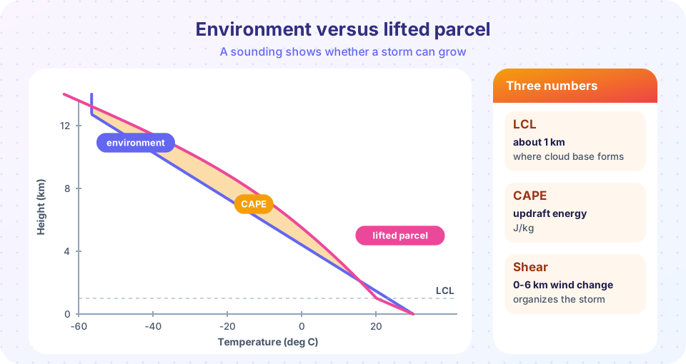
When a forecaster looks at the morning balloon sounding, three questions come to mind. How high is the cloud base? How much energy is available to a rising parcel? And does the wind change enough with height to organize storms? You can answer all three with the tools from the last two chapters. In this project you will build three synthetic days: a quiet one, a typical summer afternoon with scattered storms, and a day with an environment favorable for supercells. For each you will compute the lifting condensation level, CAPE, the 0-6 km bulk shear and a storm-risk label, and then test how sensitive the answer is to a change of a few degrees in the surface dew point. The soundings are simplified straight-line profiles, not measurements of real days, so treat the results as a classroom model.
What you will learn
- Compute LCL, LFC, equilibrium level and CAPE for a parcel lifted from the surface.
- Compute bulk shear from two wind observations.
- Combine CAPE and shear into a storm-type classification.
- Test the sensitivity of CAPE to surface moisture.
Key terms
Sounding is a vertical profile of temperature, humidity and wind. LCL is the lifting condensation level, the height where a lifted parcel saturates. LFC is the level of free convection. Bulk shear is the vector difference between the winds at two levels. Buoyancy is the upward force from a parcel being warmer than its surroundings.
The model
The parcel model is the one from the thunderstorm lesson. The environment is a straight temperature profile with a chosen lapse rate that stops cooling at −56.5 °C (a crude tropopause). The parcel starts at the surface with the surface temperature and dew point. It cools at the dry rate of 9.8 K/km up to the LCL, which is estimated as 125 × (T − Td) meters, and above it at the moist adiabatic lapse rate, which depends on temperature and pressure and which the code evaluates from physical constants at each 10 m step. Buoyancy in each layer is g (T_parcel − T_env) / T_env, and CAPE is the sum of the positive buoyancy above the LFC times the layer thickness.
The three scenarios differ in their moisture, their environmental lapse rate and their winds. Each has a surface wind and a wind at 6 km given as speed and direction.
| Day | Surface T, Td (°C) | Lapse rate (K/km) | Wind at surface | Wind at 6 km |
|---|---|---|---|---|
| A: Quiet | 22, 8 | 6.0 | 3 m/s from 180° | 8 m/s from 250° |
| B: Scattered storms | 31, 22 | 7.0 | 3 m/s from 200° | 9 m/s from 240° |
| C: Supercell setup | 29, 21 | 7.2 | 10 m/s from 160° | 30 m/s from 260° |
Press Run (or Ctrl + Enter) to see the result here.
Program input · what you'd type while the program runs
Type the answers before you press Run, one per line. Each time the program reads a line (with input()), it gets the next line from this box.
Look at the printed table. Day A has a very dry surface (a 14 degree dew point depression), so the LCL is high and the parcel never becomes buoyant. Day B has lots of CAPE but little wind change with height, so any storms that form are disorganized. Day C has both ingredients. Forecasters sum this up in an environment-based statement: instability alone does not make severe storms; shear organizes them.
Sensitivity: why moisture matters so much
CAPE is not a fixed number for a day. It is sensitive to the surface conditions, especially the dew point. A change of 2 or 3 °C in the moisture of the lowest layer, which can happen between the morning sounding and the afternoon, can double the CAPE. The second block sweeps the surface dew point for the temperature and lapse rate of Day B and plots CAPE and the LCL.
Press Run (or Ctrl + Enter) to see the result here.
Program input · what you'd type while the program runs
Type the answers before you press Run, one per line. Each time the program reads a line (with input()), it gets the next line from this box.
The curve rises steeply once the dew point is high enough that the LCL drops and the parcel stays saturated through a deep, warm layer. At low dew points the LCL is so high that the parcel arrives cold and never catches up. This is why forecasters watch the afternoon dew point so carefully and why a moist boundary layer, such as air arriving from a warm sea, is a favorite ingredient of storm days.
Reading the three days in words
A good analysis ends in sentences, not numbers. For Day A you would write that the lower atmosphere is dry and the cloud base, if any, lies near 1.7 km, that the lifted parcel never becomes warmer than its surroundings, and that no deep convection is expected whatever the trigger. For Day B you would say that the air is warm and humid, that the energy available is large, but that the winds hardly change with height, so any storms that grow will be single cells or short-lived clusters, with locally heavy rain, hail and gusty downdrafts but little organization. For Day C you would note the same instability together with strong, turning wind shear, and conclude that if storms form, they are likely to be long-lived and rotating, so watches and close radar monitoring are justified.
Notice what the analysis does not say: it does not say that storms will form. A sounding describes the environment, not the trigger. Whether a front, a sea-breeze boundary or a hill lifts the air high enough to reach the level of free convection on a given afternoon is a separate forecast, and it is the reason forecasters speak of the risk of storms and not of their certainty. In practice the sounding is only the starting point; forecasters check how the profile will change through the day with heating and moisture advection, and they compare several model runs, as you learned in the ensemble lesson.
Extensions to try
- Change the environmental lapse rate of Day B from 7.0 to 5.5 K/km and rerun. What happens to CAPE, and why?
- Find, by trial, the 0-6 km shear that moves Day B from "pulse storms" to "supercells possible" with the classify rule above. Is a speed change or a direction change cheaper in shear terms?
- Add a cap: warm the environment between 1 and 2 km by 4 °C. Does the parcel still reach the LFC? Which kind of day would a forecaster call "capped"?
- Print the theoretical maximum updraft for each day and compare with the real updrafts you learned about, which are usually about half.
Common misconceptions
"High CAPE guarantees severe storms." It guarantees only energy; storms still need a trigger, and the cap can stop everything. "Shear destroys storms." Moderate shear organizes them; only very strong shear in a weak-CAPE environment shreds them. "CAPE is measured by the balloon." It is computed from the measured profile under idealized assumptions. "A sounding from the morning predicts the afternoon." Afternoon heating and moisture changes often modify the profile substantially.
Check your understanding
Quick check · 5 questions
of 5 answered You scored / 5 · perfect!
-
1. Day A has a very dry surface. What does that do to the LCL?
LCL is about 125 m times the temperature-dew point difference, so a bigger spread gives a higher LCL. -
2. Why does Day B not produce supercells despite high CAPE?
Supercells need strong, turning shear as well as instability. -
3. Bulk shear is calculated from
Both speed and direction changes contribute, so the shear is a vector difference. -
4. If the surface dew point rises by 3 C, CAPE usually
More moisture lowers the LCL and releases more latent heat, so CAPE can rise sharply. -
5. A cap in a sounding is
A cap is a stable layer with negative buoyancy, which can prevent storms until it is broken or eroded.
Summary
- A sounding gives three key numbers for storm risk: LCL, CAPE and bulk shear.
- Instability (CAPE) is the energy; shear organizes the storm; a trigger and the lack of a cap are also needed.
- CAPE is very sensitive to the surface dew point, so moisture is a central forecast variable.
- Always compute with caution: the model is idealized and results change with the profile.
Track your progress
Create a free account to tick off lessons and pick up where you left off on any device.
of Meteorology lessons completed