


















Lesson 36 of 54 · Forecasting
Numerical weather prediction
Understand how weather models solve the equations of the atmosphere on a grid, why parametrization and data assimilation matter, and how chaos limits forecasts.
In 1922 the English mathematician Lewis Fry Richardson published a book describing how to forecast the weather by arithmetic. The idea was breathtaking: write down the laws of physics for the atmosphere, divide the globe into a grid of boxes, and calculate by hand how each box changes in the next few hours. Richardson tried it himself for a single six-hour forecast over central Europe. It took him weeks, and the result was wildly wrong: it predicted a surface pressure rise of 145 hPa in six hours, when the real pressure had barely changed. He also imagined a "forecast factory", a great hall with 64,000 human calculators, each handling one patch of the globe. Today that hall is a supercomputer, and Richardson's idea is how every weather forecast in the world is made. This lesson explains the mechanism, from the equations to the grid, and why even a perfect computer would not give a perfect forecast.
What you will learn
- List the equations behind a weather model and what they represent.
- Explain grid spacing, time steps and the cost of higher resolution.
- Describe parametrization and data assimilation.
- Demonstrate chaos with the Lorenz system.
Key terms
Numerical weather prediction (NWP) is forecasting by solving the equations of the atmosphere on a computer. Grid spacing is the horizontal distance between model points. Parametrization is a simplified representation of processes smaller than the grid. Data assimilation is the process of blending observations with a model to make initial conditions. Chaos is the extreme sensitivity of a system to its starting state.
The equations of the atmosphere
A weather model solves a small set of physical laws that you have already met in pieces.
- Momentum. Newton's second law for air: the acceleration of the wind equals the sum of the pressure gradient force, the Coriolis force, gravity and friction (the forces of chapter 5). One equation each for the east-west, north-south and vertical wind.
- Mass continuity. Air is neither created nor destroyed, so if it converges somewhere it must rise or sink.
- Thermodynamic energy. The temperature of a parcel changes with heating by the Sun, radiation, condensation and mixing, and cools as the parcel rises.
- Water. Vapor, cloud droplets, ice and precipitation are tracked, and the model keeps account of evaporation, condensation and freezing.
- Equation of state. The ideal gas law
p = ρ R Tties pressure, density and temperature together, with R = 287 J/(kg·K) for dry air.
Together these are called the primitive equations. Their solution gives wind, temperature, pressure and moisture at every point as a function of time. No one can solve them with algebra, because they are nonlinear, but a computer can step them forward in time.
Grids and time steps
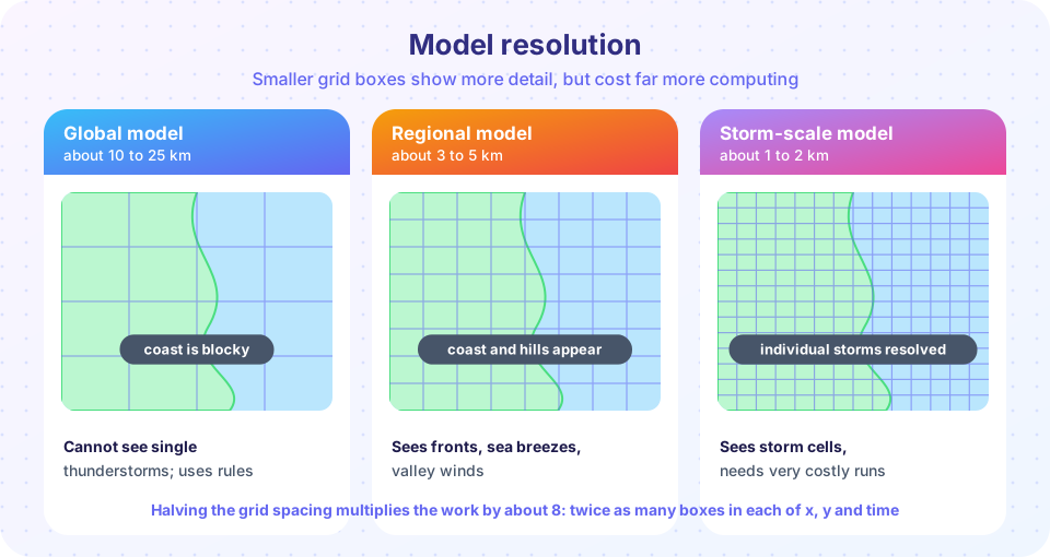
The model covers the atmosphere with a three-dimensional grid. Horizontally, the main global models use grid spacings of roughly 9 to 25 km; regional and national models use about 1 to 5 km. Vertically, there are typically between 70 and 140 layers, thin near the ground and thicker aloft. At each grid point the computer stores the variables and, over a time step of a few minutes (shorter for finer grids), calculates how each one changes from the neighboring values. Repeating this a few hundred times gives a forecast a day ahead, and a few thousand times gives ten days.
Why not simply use the finest grid possible? Because the cost grows very fast. If you halve the grid spacing, you have twice as many boxes in the east-west direction and twice as many in the north-south direction. The time step must also be halved to keep the calculation stable. Multiply the three factors and the work grows by eight. A global model that doubles its resolution therefore needs roughly eight times the computing, which is why forecast centers keep buying larger supercomputers.
Parametrization: what the grid cannot see
A thunderstorm is a few kilometers wide. A cloud droplet is a hundredth of a millimeter. Turbulent eddies near the ground are tens of meters across. None of these can be resolved on a grid of 10 km, but they matter, because they move heat, water and momentum. Models therefore include parametrizations: simplified rules that estimate the average effect of unresolved processes from the resolved variables. Typical parametrized processes are convection and cloud formation, radiation (the model calculates absorption and emission of sunlight and infrared by gases, clouds and the surface), turbulent mixing in the boundary layer, and the interaction with land, snow and sea ice. At grid spacings of about 4 km or smaller, models can start to represent big convective storms directly ("convection-permitting"), but smaller processes still require rules. Parametrization is the main source of systematic model error, and much of a model's evolution from year to year is about improving these rules.
Data assimilation
A model run is only as good as its starting point. The starting state, called the analysis, is built by data assimilation. The model's short forecast from six hours earlier, called the background or first guess, provides a complete three-dimensional picture, which is then adjusted toward the newest observations. For a single variable the idea reduces to a weighted average:
analysis = background + K × (observation − background) with K = σb² / (σb² + σo²)
where σb is the uncertainty of the background and σo the uncertainty of the observation. A precise observation gives K close to 1; a noisy one gives K close to 0. Real systems, called 4D-Var or ensemble Kalman filters, apply the same principle to hundreds of millions of variables and tens of millions of observations at once, and they use the model physics to spread the information from an observation to neighboring variables consistently. The final step after the model runs is post-processing, in which statistical methods such as Model Output Statistics correct systematic biases and interpret the output for a specific place.
Press Run (or Ctrl + Enter) to see the result here.
Program input · what you'd type while the program runs
Type the answers before you press Run, one per line. Each time the program reads a line (with input()), it gets the next line from this box.
Chaos: why the forecast has a limit
In the 1950s and 60s meteorologists hoped that more observations and bigger computers would eventually give perfect forecasts months ahead. Edward Lorenz, a meteorologist at MIT, showed in 1963 that this hope was unfounded. While running a small model of convection on an early computer, he restarted a run from a printed value that had been rounded to three decimal places and found that the new run soon diverged completely from the original. His system of three equations, now called the Lorenz system, is:
dx/dt = σ (y − x), dy/dt = x (ρ − z) − y, dz/dt = x y − β z with σ = 10, ρ = 28, β = 8/3.
It is deterministic, but two starting points that differ by a tiny amount follow trajectories that separate exponentially, so that after a while the two results are as different as two random states. This is the origin of the phrase "butterfly effect": the idea that tiny causes can have large effects later. For the real atmosphere, the practical limit of deterministic forecasts is about two weeks, because errors double roughly every day or two in the fastest-growing weather systems. Better observations and models push the limit out a little, but they cannot remove it.
Press Run (or Ctrl + Enter) to see the result here.
Program input · what you'd type while the program runs
Type the answers before you press Run, one per line. Each time the program reads a line (with input()), it gets the next line from this box.
Common misconceptions
"Forecast models are just statistical patterns from past weather." The core of a model is physics, and statistics enter only in post-processing. "A better computer would give a perfect ten-day forecast." Chaos means the error grows no matter how good the machine; better computers extend the useful range only slowly. "Weather models cannot be wrong because they use physics." Parametrization, limited resolution and imperfect initial conditions all introduce errors.
Check your understanding
Quick check · 5 questions
of 5 answered You scored / 5 · perfect!
-
1. Doubling the horizontal resolution of a model increases computing cost by about
Twice as many points in each horizontal direction and a halved time step give 2 x 2 x 2 = 8. -
2. What is parametrization?
Convection, cloud microphysics, turbulence and radiation are represented by rules based on grid-scale variables. -
3. In data assimilation, an observation with a large uncertainty receives
K = sigma_b squared over (sigma_b squared + sigma_o squared) is small when the observation is noisy. -
4. Who showed that tiny errors can grow to ruin a forecast?
Edward Lorenz's 1963 paper on deterministic nonperiodic flow introduced the sensitivity to initial conditions. -
5. Which is NOT part of the primitive equations?
The primitive equations are momentum, continuity, thermodynamic energy, moisture and the equation of state.
Summary
- Weather models solve momentum, continuity, energy, water and state equations on a grid.
- Halving the grid spacing costs about eight times as much computing.
- Parametrizations represent unresolved processes; they are a main source of model error.
- Data assimilation blends a first-guess forecast with observations by their relative uncertainty.
- Chaos limits deterministic forecasts to about two weeks and motivates ensembles.
Track your progress
Create a free account to tick off lessons and pick up where you left off on any device.
of Meteorology lessons completed