


















Lesson 50 of 54 · Projects and Practice
Project: forecast verification study
Simulate a calibrated and an overconfident forecaster, compare their Brier scores and reliability diagrams, and measure forecast value with a cost-loss model in Python.
Two weather services issue probability-of-rain forecasts for a city. Both say "70 percent" on some days and "10 percent" on others. One is honest: its 70 percent days really bring rain about 70 percent of the time. The other is overconfident: its 70 percent days bring rain only about half the time, and it says "90 percent" for events that happen much less often. On a single day you cannot tell them apart. Over a year you can. In this project you will simulate both services, score them with the Brier score, plot reliability diagrams, and then ask which forecast is more valuable to a user who has to decide whether to carry out a costly protective action. The data are simulated, with a fixed random seed, so you control the truth.
What you will learn
- Simulate forecasts and outcomes from a known true probability.
- Compute the Brier score and a Brier skill score relative to climatology.
- Build a reliability diagram from binned forecasts.
- Compare forecast value for users with different cost-loss ratios.
Key terms
Calibration (reliability) is the agreement between forecast probabilities and observed frequencies. Resolution is the ability to separate days with different outcomes. Sharpness is how far forecasts depart from the climatological frequency. Brier skill score (BSS) is the improvement over a reference forecast. Cost-loss ratio is the cost of protecting divided by the loss if the event occurs unprotected.
The simulation
We need a truth to compare with. The code gives each of 400 days a true probability of rain drawn from a skewed distribution that makes most days dry and a minority wet, as in many climates. An outcome is then drawn for each day: rain with the true probability. Two forecasters then issue their forecasts:
- Forecaster A (calibrated) knows the true probability up to a little noise and reports it, rounded to the nearest 0.05.
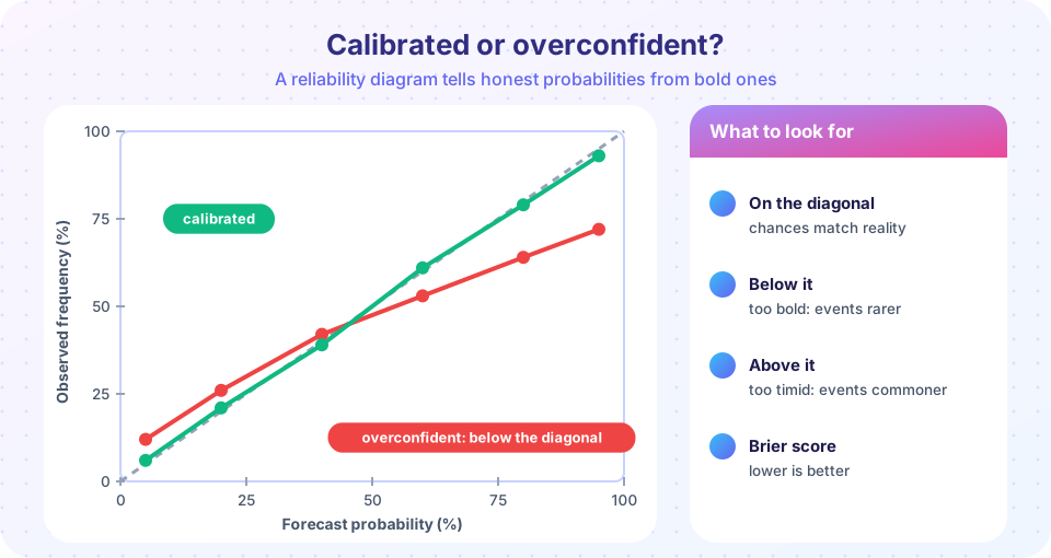
- Forecaster B (overconfident) has the same information but exaggerates it: it pushes forecasts away from the middle by tripling the "log-odds", so a true 70 percent becomes a stated 93 percent, and a true 20 percent becomes a stated 2 percent.
Notice that B has exactly the same information as A. Only the honesty differs. That makes this a clean test of calibration.
Press Run (or Ctrl + Enter) to see the result here.
Program input · what you'd type while the program runs
Type the answers before you press Run, one per line. Each time the program reads a line (with input()), it gets the next line from this box.
Study the printed scores and the diagram. The calibrated forecaster scores better (lower Brier score) and lies close to the diagonal. The overconfident forecaster has points below the diagonal at high forecast probabilities, which means that rain happened less often than stated, and the few high-probability misses cost a lot because the Brier score squares the error. Both forecasters beat climatology, because they carry real information, but B throws some of it away.
Value: who benefits more?
Verification scores treat all errors alike. A user does not. Recall the cost-loss model: a user protects (at cost C) whenever the forecast probability exceeds C/L, where L is the loss if the event happens without protection. Setting L = 1, the cost-loss ratio r = C/L ranges from 0 to 1. For a user with r = 0.1, protection is cheap and they should act on any forecast above 10 percent. For r = 0.7, they should act only when rain is likely.
The average daily expense of a user following a forecast is:
- C on every day they protect,
- L on every day they did not protect and the event occurred,
- 0 otherwise.
Compare against two references: the best a user can do with climatology alone (always protect if r is below the climatological frequency, never protect otherwise), and the expense with perfect knowledge (protect only on event days, costing climatological frequency × r). The value of a forecast is the fraction of the possible saving that it realizes:
V = (E_clim − E_forecast) / (E_clim − E_perfect)
Press Run (or Ctrl + Enter) to see the result here.
Program input · what you'd type while the program runs
Type the answers before you press Run, one per line. Each time the program reads a line (with input()), it gets the next line from this box.
The value curve is the most useful picture in verification. It shows that a forecast is not just good or bad: its usefulness depends on who is asking, and the most valuable users are those whose cost-loss ratio is close to the climatological frequency of the event, because they cannot do well with climate alone. It also shows that the damage from overconfidence is not equal across users. Look at where the two curves separate.
Reading the numbers like a forecaster
Put the results into words, because that is how a verification report is read. Both forecasters beat climatology comfortably, so both have skill. Forecaster A has a better Brier score, a reliability curve that hugs the diagonal, and a value curve that is high for nearly every user. Forecaster B's headline score is only a little worse, and a manager who looked at nothing but that one number might not notice the problem. The diagram tells the real story: on the many dry-looking days B states a chance of rain of only a few percent, and rain still happens on about one such day in seven, which is the kind of surprise that spoils a picnic or floods an unprepared basement. For a user with a very low cost-loss ratio, who protects at the smallest hint of risk, B's near-zero probabilities are worse than useless, and the value curve even dips below zero.
A word of caution about sample size. With 400 days the reliability points in the middle bins rest on only a few dozen forecasts each, so their positions wobble from one random seed to another. Real verification therefore uses years of forecasts, and confidence intervals around each point. Whenever you see a reliability diagram without any indication of how many forecasts lie behind each point, treat it as an illustration and not as proof.
Extensions to try
- Change the exaggeration factor from 3 to 1 (no exaggeration) and then to 5. At which factor does B become worse than climatology in Brier skill?
- Make a third forecaster C who is underconfident: shrink the log-odds by a factor of 0.5. Where does C's curve appear on the reliability diagram?
- Reduce the number of days from 400 to 60. How noisy do the reliability points become, and why do forecast centers need many cases?
- Make rain rarer by changing the beta distribution to
beta(0.4, 3). What happens to the climatological frequency and to the best user cost-loss ratio?
Common misconceptions
"The forecaster with the more extreme probabilities is more skilled." Sharpness is only valuable if the forecasts are also reliable. "One verification score is enough." Brier score mixes reliability and resolution; the reliability diagram and the value curve show different sides. "A forecast is good if I could act on it." Whether you can act on it depends on your cost-loss ratio.
Check your understanding
Quick check · 5 questions
of 5 answered You scored / 5 · perfect!
-
1. Forecaster B says 90% and rain happens on 60% of those days. B is
Observed frequency is lower than the stated probability, so the point lies below the diagonal. -
2. Brier skill score of 0 against climatology means
BSS = 1 - BS/BS_clim, which is zero when the Brier scores are equal. -
3. A user with C/L = 0.1 should protect when the forecast probability is
Protect when p exceeds C/L. -
4. Which forecast property is a reliability diagram designed to reveal?
It compares forecast probabilities with observed frequencies. -
5. Why does the value curve depend on the user?
Each user's optimal threshold is C/L, so the same forecast gives different benefit.
Summary
- A simulated study lets you control the truth and test verification tools.
- Calibration (reliability) and sharpness are different properties; a forecast should be both.
- The Brier score and BSS combine the properties; the reliability diagram separates them.
- Value depends on the user's cost-loss ratio, so probabilities serve more users than yes/no forecasts.
Next: Practice problems
Track your progress
Create a free account to tick off lessons and pick up where you left off on any device.
of Meteorology lessons completed