


















Lesson 39 of 54 · Forecasting
Chapter review: Forecasting
Review chapter 7 of the meteorology course with a one-page summary picture, a recap table, an error-growth simulation and a ten-question quiz on forecasting.
A modern weather forecast is the end of a long chain. Satellites, balloons, radars and thousands of stations describe the atmosphere. Data assimilation turns the patchwork into a consistent starting state. A model integrates the equations of physics forward on a grid, and an ensemble repeats the exercise many times to measure the uncertainty. Forecasters then interpret and communicate the result, and verification measures how well the whole chain performed. This review gathers the chain on one page and gives you a chance to test your grasp of it.
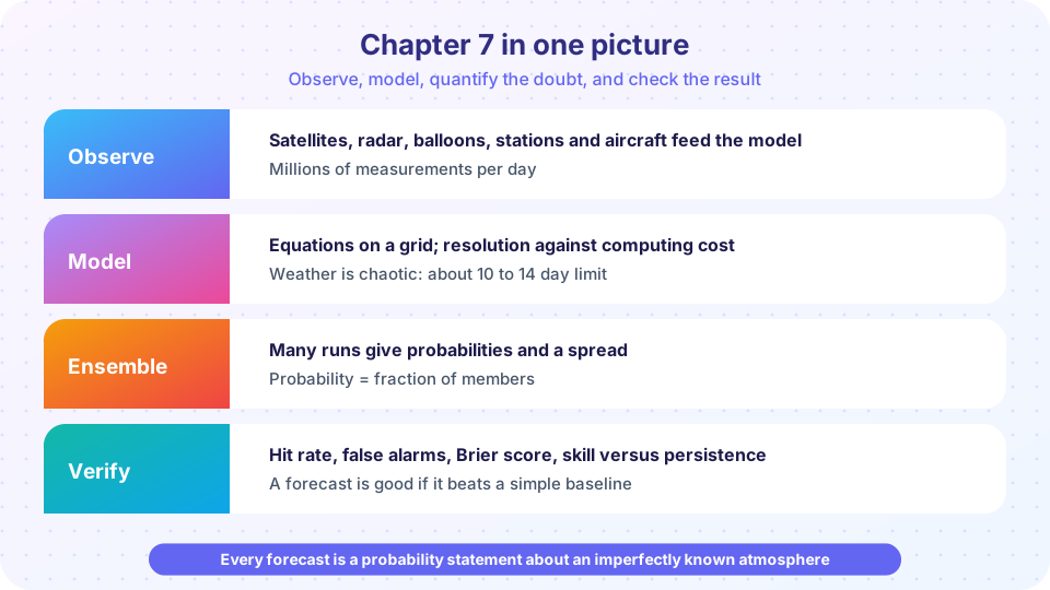
The chapter in one picture
The poster has four rows, and each row answers a question. Observe: what is the atmosphere doing now? Model: what do the laws of physics say will happen next? Ensemble: how much should we trust that answer? Verify: was it good, and good compared with what? Notice that uncertainty runs through all of them: the observations are imperfect, the model is approximate, chaos amplifies the errors, and verification must account for what a forecast would have scored by luck.
Recap table
| Topic | Key facts |
|---|---|
| Observations | Surface stations, radiosondes (00 and 12 UTC), radar, satellites, aircraft, buoys |
| Satellites | Geostationary at 35,786 km (constant view); polar at 800-850 km (about 14 orbits/day) |
| Radar | Reflectivity in dBZ; Z = 200 R^1.6; Doppler velocity shows rotation |
| Station model | Pressure code 132 = 1013.2 hPa, 875 = 987.5 hPa; barb: 5 / 10 / 50 kt |
| Numerical prediction | Primitive equations on a grid; cost rises about 8x when spacing halves |
| Parametrization | Rules for convection, clouds, radiation and turbulence that the grid cannot resolve |
| Data assimilation | analysis = background + K (obs − background), K = σb² / (σb² + σo²) |
| Chaos | Lorenz 1963; small errors double in about a day or two; about two weeks of range |
| Ensembles | 20 to 50 runs from perturbed starts; probability = fraction of members |
| PoP | Chance of measurable rain; in the US, confidence times area fraction |
| Verification | POD, FAR, bias, CSI, Brier score, skill versus persistence or climatology |
| Value | Act when probability exceeds the cost-loss ratio C / L |
Try it
The simulation below is an idealized sketch, not a real forecast model. It lets forecast error grow by a fixed doubling time and saturate at the level of climatology, the error you would make by always forecasting the average. The point where the forecast error approaches the climatological error is the practical limit of predictability. Try different doubling times and initial errors.
Press Run (or Ctrl + Enter) to see the result here.
Program input · what you'd type while the program runs
Type the answers before you press Run, one per line. Each time the program reads a line (with input()), it gets the next line from this box.
You should find that halving the initial error extends the range by only about a day and a half in this model: with a doubling time of 1.5 days, cutting the starting error in half is the same as shifting the curve by exactly one doubling time. That is a good picture of why forecast improvements come slowly even though instruments and computers have improved enormously.
Common misconceptions
"If the model is physics, forecasts should eventually be perfect." Chaos sets a limit that better instruments only stretch slowly. "A single deterministic run is the forecast." Operational forecasts combine many runs, a forecaster's judgment and statistical correction. "Verification is just counting how often the forecast was right." Good verification uses several scores, baselines and many cases.
Check your understanding
Quick check · 10 questions
of 10 answered You scored / 10 · perfect!
-
1. Which observing platform provides a continuous view of one hemisphere?
A geostationary satellite stays above one point on the equator and images the same disk continuously. -
2. Station-model pressure code 982 means
982 is 500 or more, so prefix 9: 9982, which is 998.2 hPa. -
3. A radar reflectivity of 40 dBZ corresponds approximately to a rain rate of
Z = 10,000, and (10,000 / 200)^(1/1.6) is about 11.5 mm per hour. -
4. Doubling the resolution of a model increases the cost by about
Two more points in each horizontal direction and a halved time step give a factor of eight. -
5. In data assimilation, K close to 1 means
K is the weight on the observation; it is near 1 when the observation is much more accurate than the background. -
6. What did Lorenz show in 1963?
His three-equation model has trajectories that diverge exponentially from nearby starts. -
7. 15 of 30 ensemble members forecast snow. The probability is
15 / 30 = 0.5. -
8. The hurricane forecast cone shows
The cone is built from past track errors; impacts extend beyond it. -
9. A user has a cost-loss ratio of 0.2. They should protect when the probability is above
Protect if p > C/L = 0.2. -
10. Why can percent correct be a poor score for rare events?
Correct negatives dominate when events are rare, so a forecast with no skill can score well.
Summary
- Forecasting chains observation, assimilation, simulation, ensembles, interpretation and verification.
- Resolution costs grow about eightfold per halving of grid spacing; parametrization handles small processes.
- Chaos limits deterministic forecasts to about two weeks, so probabilities are essential.
- Verification uses contingency scores, the Brier score and skill against a baseline, and value depends on the user.
- The next chapter applies these tools to severe weather and climate connections.
Track your progress
Create a free account to tick off lessons and pick up where you left off on any device.
of Meteorology lessons completed