


















Lesson 47 of 51 · Projects and Practice
Project: Hunting for the Higgs Bump
Simulate a diphoton mass spectrum, fit the background, measure the significance of a signal with a likelihood ratio, and estimate the look-elsewhere effect with toy experiments.
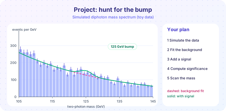
The Higgs boson was found as a small bump in the distribution of the invariant mass of photon pairs (and of four-lepton combinations). In this project you will rebuild the logic of that search with simulated data. You will generate a mass spectrum, fit a smooth background, fit a signal on top, compute the significance, and finally account for the fact that you looked at many places, the look-elsewhere effect.
Everything here is a toy simulation, with made-up event counts and a simplified shape, to practice the method. It is not real LHC data.
What you will learn
- How to simulate counting data with Poisson fluctuations.
- How to fit a background and a signal with a likelihood.
- How to compute a significance from the likelihood ratio.
- What the look-elsewhere effect is and how to estimate it with toys.
- How the quoted "5σ" differs from the local significance of a single bump.
Key terms
Poisson likelihood: the probability of the observed bin counts given expected counts: L = ∏ μᵢ^nᵢ e^(−μᵢ) / nᵢ!.
Likelihood ratio q₀ = −2 ln (L_background / L_signal+background): a test statistic; for large samples Z = √q₀ is the significance in standard deviations.
Local significance: the significance at a mass fixed in advance.
Global significance: the significance after accounting for the whole range that could have shown a bump.
Toy experiment: a pseudo-dataset drawn from a model, used to find the distribution of a statistic.
Step 1: simulate the spectrum and fit
We use 1 GeV bins between 105 and 160 GeV. The background falls exponentially, B(m) = A e^(−(m−105)/τ) with A = 2200 events per GeV and τ = 30 GeV. The signal is a Gaussian of width 1.7 GeV (a typical detector resolution) at 125 GeV with 450 events in total.
Press Run (or Ctrl + Enter) to see the result here.
Program input · what you'd type while the program runs
Type the answers before you press Run, one per line. Each time the program reads a line (with input()), it gets the next line from this box.
Step 2: scan the mass
If you did not know the mass in advance, you would scan: for each hypothesis m_H, fit the signal strength and compute the local significance. The plot of significance versus mass shows the bump, but also random fluctuations elsewhere.
Press Run (or Ctrl + Enter) to see the result here.
Program input · what you'd type while the program runs
Type the answers before you press Run, one per line. Each time the program reads a line (with input()), it gets the next line from this box.
Step 3: the look-elsewhere effect
If a spectrum is pure background, scanning 46 hypotheses makes it likely that at least one will show an upward fluctuation of 2σ to 3σ. Such a peak is a fluke, not a particle. To find how big the biggest fluke is likely to be, generate many background-only toys, scan each, and record the largest significance. The fraction of toys that exceed your observed value is the global p-value.
To keep the calculation fast we use a linearized signal estimator: for each hypothesis, ŝ = Σ(nᵢ − bᵢ)gᵢ/bᵢ / Σgᵢ²/bᵢ, with Z = ŝ / σ_ŝ, where gᵢ is the normalized signal shape and bᵢ the fitted background.
Press Run (or Ctrl + Enter) to see the result here.
Program input · what you'd type while the program runs
Type the answers before you press Run, one per line. Each time the program reads a line (with input()), it gets the next line from this box.
Reading your results
- A single bump at a mass you chose in advance has a local significance. The same bump found by scanning has a lower global significance.
- The real Higgs result was announced with a local significance of about 5σ in each of the two experiments' combined channels. The global significance was somewhat lower, which is why experiments waited for more data and independent channels before using the word "discovery".
- Real analyses add many details: different decay channels, systematic uncertainties on the background shape, detector resolution that depends on where the photons hit, and thousands of simulated events to build the signal model.
Extensions
- Make the background shape a polynomial instead of an exponential and see how the significance depends on the choice (a systematic uncertainty).
- Change the signal to 200 events. How much more data would you need to reach 5σ? (Hint:
Z ∝ √Nwhen S/B stays fixed.) - Add a second, wider peak (a different resolution category) and fit both.
Common misconceptions
"A 3σ peak means 99.7% probability that the particle exists." It means the background alone would give an excess this big with a probability of about 0.13% at that fixed place. It is not the probability of the hypothesis.
"We can pick the best-looking bump and quote its local significance." The look-elsewhere effect makes that biased; global significance is lower.
"The fit proves the shape is right." The significance depends on the assumed background shape. A bad shape can create or hide bumps, so analysts test several.
Check your understanding
Quick check · 5 questions
of 5 answered You scored / 5 · perfect!
-
1. What does the likelihood ratio q₀ compare?
q₀ = −2 ln(L_b/L_sb); a large value means the signal hypothesis describes the data much better. -
2. A bump found by scanning 46 mass hypotheses has a lower global significance than local because...
That is the look-elsewhere effect. -
3. If the signal and background both doubled with the same ratio S/B, the significance would roughly...
Z ∝ S/√B ∝ √N when S/B is fixed. -
4. Why simulate toy experiments?
Toys show how often fluctuations of a given size occur. -
5. What are the bin contents in this simulation drawn from?
Counting experiments fluctuate according to Poisson statistics.
Summary
- A bump search compares a background-only fit with a signal-plus-background fit using a Poisson likelihood.
Z = √q₀gives the local significance; discovery needs about 5σ (p ≈ 3×10⁻⁷).- Scanning many masses causes the look-elsewhere effect, which lowers the global significance.
- Toy experiments give the distribution of the largest fluctuation without a signal.
- Real analyses must also treat the background-shape systematics.
Track your progress
Create a free account to tick off lessons and pick up where you left off on any device.
of Nuclear and Particle Physics lessons completed