


















Lesson 42 of 49 · Observation and Modelling
Chapter 8 Review: Observation and Modelling
Review chapter 8: CTD, Argo, moorings, satellite altimetry and geostrophic currents, grid resolution, the CFL limit, data assimilation and two-layer heat uptake, with a ten-question quiz.
Chapter 8 showed how people learn about an ocean they cannot see. They lower instruments from ships, leave robots to drift, listen to the sea from orbit and then run the laws of physics forward on computers. None of these approaches is enough alone. The skill of an oceanographer is to know what each source can and cannot say, and to combine them.
What you will learn
- The key numbers and formulas of chapter 8
- How the observing system and the models fit together
- Which ideas to revisit before the projects in chapter 9
Key terms
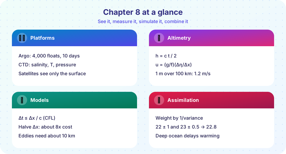
Argo: about 4,000 floats; 10-day cycles; profiles to 2,000 m.
Altimetry: h = c t / 2; sea level slope gives u = (g/f)(Δη/Δx).
CFL condition: c Δt / Δx ≤ 1, with c = √(gH) for the fastest wave.
Assimilation: x_a = (x_b/σ_b² + y/σ_o²) / (1/σ_b² + 1/σ_o²).
Two-layer model: surface warming lags equilibrium F/λ because of the deep ocean's heat capacity.
Recap table
| Lesson | Core idea | Formulas and numbers |
|---|---|---|
| Chapter 8 Overview | No single platform sees everything | About 146,000 Argo profiles a year; about 300 km per float |
| Ships, Floats and Satellites | Each platform has a niche; satellites see only the surface | h = ct/2; round trip 8.9 ms from 1,336 km; 1 m over 100 km at 35°N gives 1.2 m/s |
| Models and Data | Equations on a grid, corrected by data | Rossby radius 10 to 200 km; halving Δx costs about 8 times more; Δt ≤ Δx/c |
How the pieces connect
The chapter can be read as a loop. Instruments sample the ocean in situ and from space; the data are checked, calibrated and combined; a model fills the gaps between the samples by solving the physical equations; and the improved picture shows where more or better measurements are needed. Each link has a number you can compute: how many profiles a float array collects, how fast a radar pulse returns, how steep a sea surface slope gives a certain current, how long a model time step may be and how to weigh a forecast against an observation. Understanding these numbers lets you judge both the strengths and the limits of ocean science.
Common misconceptions
"Satellites see the deep ocean." They sense only the surface layer.
"Models are guesses." They solve physical laws and are tested against data.
"Finer resolution is always better." It costs far more and cannot fix wrong physics.
"Argo tracks floats continuously." Floats are located only when they surface.
Try it
The first example is a formula drill for the chapter.
Press Run (or Ctrl + Enter) to see the console output here.
No output.
The second example plots how the geostrophic current for a fixed sea level slope changes with latitude. The current grows toward the equator because the Coriolis parameter shrinks, which also shows why geostrophy stops working very close to the equator.
Press Run (or Ctrl + Enter) to see the result here.
Program input · what you'd type while the program runs
Type the answers before you press Run, one per line. Each time the program reads a line (with input()), it gets the next line from this box.
Check your understanding
Quick check · 10 questions
of 10 answered You scored / 10 · perfect!
-
1. Which instrument measures conductivity, temperature and pressure through the water column?
CTD stands for conductivity, temperature and depth. -
2. About how far apart are Argo floats?
4,000 floats over 361 million km² gives about 90,000 km² each, a square with a side of about 300 km. -
3. A radar altimeter measures distance as...
The pulse goes down and back, so the one-way distance is half of c times the round-trip time. -
4. Which is NOT measurable directly from satellites?
Satellites sense only the surface layer. -
5. What does the CFL condition limit?
c Δt / Δx must not exceed 1 for explicit schemes. -
6. Why does a finer grid cost much more computing?
Four times as many cells in the horizontal and twice as many steps. -
7. Model 20.0 ± 2.0 °C and observation 22.0 ± 1.0 °C give an analysis closest to...
Weights 1/4 and 1: (20×0.25 + 22×1)/1.25 = 21.6. -
8. What is the main role of a parameterization?
Parameterizations capture the net effect of processes smaller than the grid. -
9. Why does geostrophic balance not work right at the equator?
f = 2Ω sin φ is zero at φ = 0, so u = (g/f)(Δη/Δx) is not valid. -
10. In the two-layer model, the surface warms to the equilibrium F/λ...
The deep ocean's large heat capacity delays the final warming.
Summary
- Ships, moorings, floats, gliders and satellites each sample different scales; the observing system combines them.
- Satellites see the surface: altimetry gives height and, with geostrophy, currents; the interior needs in situ data.
- Models solve the primitive equations on a grid; resolution and the CFL condition set the computing cost.
- Assimilation blends data and model by their uncertainties; simple models such as the two-layer one illustrate key results.
- Chapter 9 puts these ideas to work in projects and practice.
Track your progress
Create a free account to tick off lessons and pick up where you left off on any device.
of Oceanography lessons completed