


















Lesson 41 of 49 · Observation and Modelling
Models and Data
Learn how ocean models work: equations on a grid, resolution and the Rossby radius, the CFL time step, parameterization, data assimilation, and a two-layer model of ocean heat uptake.
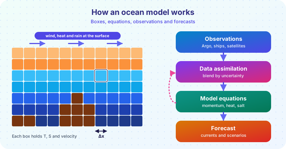
An oceanographer who wants to know where a spilled drum of oil will end up in ten days, what a hurricane will do to the water it crosses or how much heat the ocean will take up in this century cannot simply run an experiment. The ocean cannot be put in a laboratory. The tool of choice is the numerical model: a computer program that represents the ocean as a grid of boxes and steps the laws of physics forward in time.
This lesson explains what such a model contains, why its resolution matters, how a model is corrected with observations, and how a very simple model already explains an important feature of the climate: why the ocean delays warming. It also shows how to judge a model fairly, by knowing what it can and cannot do.
What you will learn
- What equations an ocean model solves
- Why grid spacing matters, and what the Rossby radius has to do with it
- What the CFL condition limits, with a worked time-step calculation
- What parameterization and data assimilation are, with a simple example of each
- How a two-layer model explains slow ocean warming
Key terms
Grid cell: one box of the model, holding a single value of temperature, salinity and velocity for each variable.
Resolution: the size of a grid cell; smaller cells show finer features but cost more computing.
Parameterization: a simplified rule that represents the effect of processes too small or too complicated to simulate directly.
Data assimilation: the statistical blending of observations with a model forecast to get the best estimate.
Ensemble: a set of model runs with slightly different starts or settings, used to estimate uncertainty.
What goes into a model
Most ocean models solve a set of equations called the primitive equations:
- Momentum: Newton's second law for a rotating fluid. The acceleration of a parcel equals the pressure gradient, the Coriolis force, gravity, wind stress and friction.
- Continuity: water is conserved (the flow is nearly incompressible).
- Heat and salt conservation: temperature and salinity are carried by the flow and changed by mixing and by exchange at the surface.
- Equation of state: density as a function of temperature, salinity and pressure (chapter 3).
- Hydrostatic balance: pressure increases with depth in proportion to the weight of the water above.
The program divides the ocean into a three-dimensional grid, typically 30 to 100 vertical layers, and advances these equations in small steps of time, with wind, heat and freshwater at the surface supplied by atmospheric data or by a coupled atmosphere model. A global model with 10 km boxes has hundreds of millions of cells and runs on supercomputers.
Resolution and the Rossby radius
What features can a model show? A rule of thumb is that it must have at least two or three grid cells across a feature in order to represent it. The key length for ocean eddies is the Rossby radius of deformation, about 30 to 50 km at mid-latitudes, 10 km or less near the poles, and 200 km or more near the equator. Eddies of this size, which stir heat and carbon through the ocean, need grid spacing of about 10 km (0.1 degrees) or less. Climate models running for centuries often use 1 degree (about 100 km) in the ocean, which does not resolve eddies. Instead the model includes a parameterization: a formula, such as the 1990 Gent-McWilliams scheme, that represents the net effect of the missing eddies.
Resolution has a steep cost. Halving the grid spacing in both horizontal directions gives four times as many cells, and the time step must be halved too, so the computing cost goes up by a factor of about 8. Going from 100 km to 10 km multiplies the cost by roughly 1,000.
The time step
Numerical stability limits how long each step can be. In an explicit scheme the fastest wave in the model must not travel more than one grid cell per step. This is the CFL condition (after Courant, Friedrichs and Lewy): c Δt / Δx ≤ 1. The fastest wave in the ocean is the surface gravity wave of the whole water column with speed c = √(g H). For H = 4,000 m, c = 198 m/s. With Δx = 10 km:
Δt ≤ Δx / c = 10,000 / 198 ≈ 50 s
Modelers use tricks (splitting the fast surface waves from the slow internal ones) to take longer steps for the bulk of the computation, but the idea remains: finer grids need shorter time steps.
Observations meet models: data assimilation
A model started from an estimate of the ocean drifts away from the real ocean, because small errors grow and because the model's physics are imperfect. Observations pull it back. The simplest case shows the idea. Suppose the model forecasts a sea temperature of x_b with an error variance σ_b², and an observation y has an error variance σ_o². The best combined estimate weights each by the inverse of its variance:
x_a = (x_b / σ_b² + y / σ_o²) / (1 / σ_b² + 1 / σ_o²), with 1 / σ_a² = 1 / σ_b² + 1 / σ_o²
If the model says 22.0 °C ± 1.0 and a float says 23.0 °C ± 0.5, the analysis is (22/1 + 23/0.25) / (1 + 4) = 22.8 °C, with an error of 0.45 °C: closer to the more accurate source, and more certain than either. Operational systems extend this logic to millions of variables and observations at once, using methods such as the Kalman filter and variational (4D-Var) assimilation. They run daily at national centers to produce ocean forecasts, and reanalyses use the same machinery to rebuild the past ocean as a smooth, complete data set.
What models are used for
- Forecasts: currents for search and rescue, ship routing, oil spill tracking and harbor management; also seasonal ENSO forecasts from coupled models.
- Climate projections: Earth system models couple ocean, atmosphere, ice and biogeochemistry to explore different emission scenarios.
- Process studies: switch off one factor, such as the wind, and see what changes, which is something nature does not allow.
- Filling gaps: interpolate between observations.
A two-layer model of ocean heat uptake
Even a very simple model teaches something real. Treat the climate as a thin upper layer (the atmosphere, land and ocean mixed layer, with heat capacity C) over a large deep ocean (heat capacity C_d). A forcing F (for doubled carbon dioxide, about 3.7 W/m²) warms the upper layer to a temperature anomaly T. The layer loses heat to space at a rate λ T and to the deep ocean at γ (T − T_d):
C dT/dt = F − λ T − γ (T − T_d)
C_d dT_d/dt = γ (T − T_d)
With λ = 1.2 W/m²/K, the final warming would be F / λ = 3.1 K. But the upper layer responds in only a few years, while the deep ocean takes centuries to catch up, so the warming is delayed. The surface temperature climbs fast at first and then creeps up slowly. This is the thermal inertia of the ocean, and it means that part of the warming caused by past emissions has not appeared yet.
Judging a model
A model is a tool, not a crystal ball. Modelers compare their output with observations (bias, root-mean-square error and skill relative to a simple forecast), test across many situations and run ensembles to show uncertainty. Known weaknesses include poorly resolved eddies, mixing in the deep ocean, the shape of the Gulf Stream and the Antarctic coast, and the representation of sea ice and biology. A model should be trusted for what it has been shown to do well: for example, the large-scale heat uptake is robust, but the behavior of a single small eddy is not.
Common misconceptions
"A model predicts the future exactly." A model gives a range of outcomes, depending on the scenario and uncertainty.
"Higher resolution is always better." It is better for features of that size, but it costs far more, and it cannot fix wrong physics.
"Models are tuned to give the answer wanted." Parameters are chosen to match observations, and the results are then tested against data not used in the tuning.
"Assimilation just replaces the model with data." It blends them by their uncertainties.
Try it
The first example shows two core calculations: how to combine a model forecast with an observation (data assimilation for a single number) and the maximum time step permitted by the CFL condition.
Press Run (or Ctrl + Enter) to see the console output here.
No output.
The second example integrates the two-layer model for 500 years after a sudden doubling of carbon dioxide. The parameters are standard textbook values for a simple energy-balance model. It is a teaching model with no geography, not a forecast.
Press Run (or Ctrl + Enter) to see the result here.
Program input · what you'd type while the program runs
Type the answers before you press Run, one per line. Each time the program reads a line (with input()), it gets the next line from this box.
Check your understanding
Quick check · 5 questions
of 5 answered You scored / 5 · perfect!
-
1. Why do climate models often use 1-degree ocean grids?
Cost grows steeply as the grid shrinks, so long climate runs trade resolution for length and ensembles. -
2. A model has a 4,000 m deep ocean (c = 198 m/s) and 10 km grid spacing. The CFL limit on an explicit time step is about...
Δt ≤ Δx / c = 10,000 / 198 ≈ 50 s. -
3. What does a parameterization do?
Parameterizations stand in for processes, such as eddies or turbulence, that the grid cannot show. -
4. Model 20.0 ± 1.0 °C, observation 21.0 ± 1.0 °C. The analysis is...
Equal errors give equal weights: 20.5 °C, with error σ/√2 ≈ 0.71 °C. -
5. In the two-layer model, why does surface warming lag behind the equilibrium?
Heat flowing into the deep ocean slows the warming of the upper layer.
Summary
- Ocean models solve the primitive equations (momentum, continuity, heat, salt, equation of state) on a grid.
- Resolution matters: eddies need about 10 km spacing; halving the grid costs about 8 times more; the CFL condition
Δt ≤ Δx/climits the time step. - Parameterizations stand in for unresolved processes; data assimilation blends model and observations by their uncertainties.
- Even a two-layer model shows that the deep ocean's heat capacity delays surface warming by decades to centuries.
- Models should be judged against observations and used for what they do well.
Track your progress
Create a free account to tick off lessons and pick up where you left off on any device.
of Oceanography lessons completed