


















Lesson 29 of 48 · Transportation Engineering
Traffic flow fundamentals
Learn the three variables of traffic flow, the Greenshields model, lane capacity, level of service and why a brake light can start a traffic jam.
Anyone who has sat in a traffic jam with no visible cause has met the subject of this lesson. Traffic behaves like a fluid: cars are the particles, the road is the pipe, and there are simple relationships between how many cars are on the road, how fast they move and how many pass per hour. Engineers use those relationships to plan lanes, time signals and predict when a road will break down.
What you will learn
- How flow, density and speed are related by q = k v.
- How the Greenshields model predicts capacity and the optimal density.
- How headway and spacing connect to flow.
- How a shock wave moves through a queue.
Key terms
Flow (q): vehicles per hour passing a point. Density (k): vehicles per kilometer on a stretch of road. Space-mean speed (v): the average speed of vehicles on a stretch of road. Jam density (k_j): the density at which traffic stops, typically around 120 to 150 vehicles per km per lane for cars. Capacity: the maximum flow a road can sustain.
The basic relation
Imagine standing beside a road and counting cars. If there are k vehicles in each kilometer and they all travel at v km/h, then in one hour the cars from the previous v kilometers pass you:
q = k v
Example: 25 veh/km at 80 km/h gives 2000 veh/h. The same flow can happen in two very different states: a light, fast stream, or a dense, slow one. That is the point of the next section.
The Greenshields model
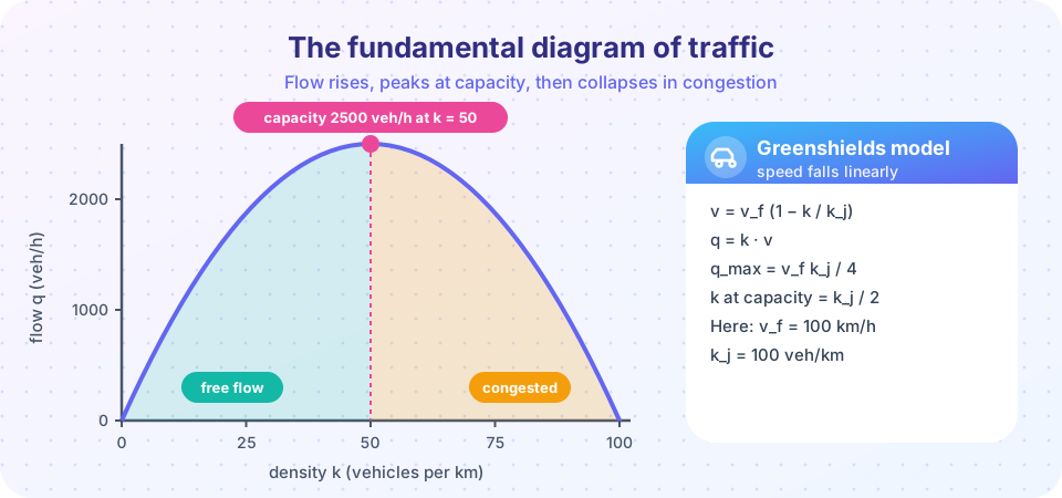
In 1935 Bruce Greenshields measured traffic and proposed that speed falls linearly with density, from the free-flow speed v_f at k = 0 to zero at the jam density k_j:
v = v_f (1 − k / k_j)
Substituting into q = k v gives a parabola:
q = v_f k (1 − k / k_j)
The peak is found by setting the derivative to zero. It occurs at k = k_j / 2 and equals q_max = v_f k_j / 4. With v_f = 100 km/h and k_j = 100 veh/km, the capacity is 100 × 100 / 4 = 2500 veh/h at k = 50 veh/km and v = 50 km/h.
Two points on the curve have the same flow: at k = 30, q = 30 × 70 = 2100, and at k = 70, q = 70 × 30 = 2100. The first is free flow and the second is congested. Once density passes the peak, more cars means fewer cars per hour. This is why a road "breaks down" suddenly: a small increase in demand pushes it across the peak and flow collapses.
Real roads are not perfect parabolas, and the highest observed lane flows are somewhat different, but the model teaches the key lesson. Modern manuals report lane capacities of the order of two thousand passenger cars per hour for freeways.
Headway and spacing
Two measures describe the gap between vehicles. Time headway h is the time between successive vehicles passing a point, and spacing s is the distance between them. They connect to the flow and density: q = 3600 / h (veh/h, h in seconds) and k = 1000 / s (veh/km, s in meters). A 2-second headway is 1800 veh/h. Safe-driving rules often recommend a gap of two seconds because it gives the driver time to react.
Level of service
Because flow alone does not tell how the trip feels, the Highway Capacity Manual and other guides grade conditions from A (free flow) to F (stop-and-go) using density, speed or delay. LOS A to C describes comfortable conditions, D and E are increasingly crowded, and F means demand exceeds capacity. Planners often design for LOS C or D.
Shock waves
When fast traffic meets a slow queue, the boundary between them moves like a wave. If state 1 has flow q₁ and density k₁ and state 2 has q₂ and k₂, the wave speed is
w = (q₂ − q₁) / (k₂ − k₁)
Take free flow at k₁ = 30 veh/km (q₁ = 2100 veh/h) and a queue at k₂ = 80 veh/km (q₂ = 1600 veh/h). Then w = (1600 − 2100) / (80 − 30) = −10 km/h. The negative sign means the end of the queue moves backward, upstream at 10 km/h, while every car in it still moves forward. This is the "phantom jam": a driver who brakes slightly makes the car behind brake harder, and the disturbance travels backward as a wave.
Common misconceptions
"Flow is highest when traffic is fastest." Flow peaks at moderate speed and moderate density. At very high speed the cars are far apart and few pass per hour.
"Congestion means cars have stopped moving forward." In a jam the cars move; it is the congested region that moves backward.
"Greenshields predicts exact flows." It is a simple model. Real roads need local data for v_f, k_j and capacity.
Try it
The first demo draws all three views of the fundamental diagram. The second computes shock-wave speeds for any two states.
Press Run (or Ctrl + Enter) to see the result here.
Program input · what you'd type while the program runs
Type the answers before you press Run, one per line. Each time the program reads a line (with input()), it gets the next line from this box.
Press Run (or Ctrl + Enter) to see the console output here.
No output.
Check your understanding
Quick check · 5 questions
of 5 answered You scored / 5 · perfect!
-
1. A road has 40 veh/km moving at 60 km/h. What is the flow?
q = k v = 40 × 60 = 2400 veh/h. -
2. With the Greenshields model, at what density is the flow highest?
Setting dq/dk = 0 gives k = k_j / 2. -
3. If v_f = 120 km/h and k_j = 100 veh/km, the Greenshields capacity is
q_max = v_f k_j / 4 = 120 × 100 / 4 = 3000 veh/h. -
4. A shock wave speed of −10 km/h means the queue end
A negative wave speed means the boundary travels against the direction of traffic. -
5. A 1.5-second headway corresponds to a lane flow of
q = 3600 / 1.5 = 2400 veh/h.
Summary
- Flow, density and speed are related by
q = k v. - Greenshields:
v = v_f (1 − k/k_j), capacityv_f k_j / 4atk_j / 2. - Headway and spacing convert to flow and density.
- Level of service grades road conditions from A to F.
- Shock waves in queues travel upstream.
Next: Geometric design
Track your progress
Create a free account to tick off lessons and pick up where you left off on any device.
of Civil Engineering Fundamentals lessons completed