


















Lesson 45 of 48 · Projects and Practice
Project: a dosing regimen simulator
Build a Python model of drug concentration with repeated oral doses, test it against a therapeutic window, and add kidney disease and an interacting drug.
Drug companies, hospital pharmacists and researchers all use models to ask "what if". What if the dose is halved? What if the patient's kidneys clear the drug at half the usual rate? What if a second drug slows the liver enzyme that removes it? In this project you will build a small simulator that answers such questions. You will start from one equation, extend it to repeated doses, compare regimens against a therapeutic window and finish with a tool that tests several scenarios side by side. Everything runs in your browser. The drug is imaginary and the numbers are chosen for teaching, so the project shows the method, not advice for any real medicine.
Educational information only. The model is a simplified teaching tool. Real dosing uses measured patient data, validated models and clinical judgment. Do not use this simulator to choose a dose for a person.
What you will learn
- Write the one-compartment oral absorption model and explain each parameter.
- Use superposition to model repeated doses.
- Measure peak, trough, average level and time in the therapeutic window.
- Explore how reduced clearance and a drug interaction change the result.
Key terms
One-compartment model: a simplification in which the body behaves as a single well-mixed volume with first-order elimination.
Absorption rate constant (ka): how quickly an oral dose enters the blood, per hour.
Elimination rate constant (ke): the fraction of drug removed per hour, equal to CL divided by Vd.
Superposition: adding the contributions of each dose, valid when the kinetics are linear.
Trough and peak: the lowest and highest levels between doses.
The model
Assume the body is one compartment of volume V (liters). A dose D (mg) is swallowed. A fraction F (bioavailability) is absorbed, at a rate that is proportional to the amount still in the gut: first-order absorption with constant ka. The drug is removed from the blood at a rate proportional to its concentration, first-order elimination with constant ke = CL / V, where CL is clearance in liters per hour. The concentration at time t after a single dose is then
C(t) = F·D·ka / (V·(ka − ke)) × (e^(−ke·t) − e^(−ka·t))
The two exponentials are the rise and the fall. Early on, absorption dominates, and the curve climbs. Later, elimination dominates and it declines. The time of the peak, tmax, comes from setting the slope to zero: tmax = ln(ka/ke) / (ka − ke). Three other relations are worth remembering:
- Half-life
t½ = ln 2 / ke = 0.693 × V / CL. - For repeated doses every
τhours at steady state, the average concentration isCss,avg = F·D / (CL·τ). The total amount in per interval equals the amount out. - The accumulation ratio
R = 1 / (1 − e^(−ke·τ))tells you how much higher the steady-state trough is than the level just after the first dose's decay. When τ equals the half-life, R = 2.
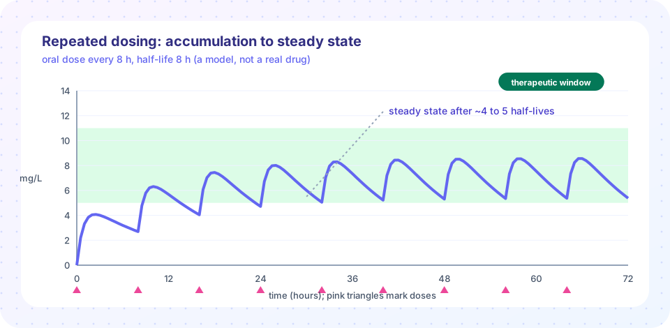
Because the model is linear, if you give a second dose at time τ, its curve starts at τ and adds to the first. That is superposition: you simply sum shifted copies of the single-dose curve. The simulation in the third step does exactly this.
Step 1: one dose
Start with the single-dose function and look at the curve. Try changing ka to see how faster absorption gives a higher, earlier peak, and change the clearance to see how the tail changes.
Press Run (or Ctrl + Enter) to see the result here.
Program input · what you'd type while the program runs
Type the answers before you press Run, one per line. Each time the program reads a line (with input()), it gets the next line from this box.
Step 2: repeated doses and the therapeutic window
Now add superposition. The function sums the single-dose curves, one per dose. Then it measures three numbers over the last dosing interval: the peak, the trough and the percentage of time inside a therapeutic window of 5 to 11 mg/L. The window is made up for this imaginary drug.
Press Run (or Ctrl + Enter) to see the result here.
Program input · what you'd type while the program runs
Type the answers before you press Run, one per line. Each time the program reads a line (with input()), it gets the next line from this box.
Notice how the two regimens give the same daily dose and the same average level, but different swings. Splitting the dose into smaller, more frequent amounts narrows the range between peak and trough. That is the reason for slow-release tablets and for splitting the dose of drugs with a narrow therapeutic index.
Step 3: the full tool with scenarios
The last step wraps everything into a table of scenarios. It models the baseline, a patient with kidney disease whose clearance is halved, the same patient after a dose reduction, and a patient whose liver enzyme is inhibited by another drug so that clearance falls to 40 percent. These multipliers are invented to show the pattern. For each scenario the tool prints the average, peak and trough and flags levels above the window.
Press Run (or Ctrl + Enter) to see the result here.
Program input · what you'd type while the program runs
Type the answers before you press Run, one per line. Each time the program reads a line (with input()), it gets the next line from this box.
The output makes the lesson of the case studies concrete. Halving clearance doubles the average level, because Css,avg = F·D / (CL·τ). Halving the dose brings it back. The enzyme inhibitor case pushes the level much higher still. In real practice, doses are adjusted using measured kidney function and, for narrow-index drugs, measured blood levels.
Checking your model
A simulator is only useful if you trust it, so test it against things you can calculate by hand. Run a single intravenous-like case by making ka very large: the peak should be close to dose / Vd. Check that the average level over a long run matches F·D / (CL·τ). Verify that doubling V while keeping CL fixed doubles the half-life, and that doubling the dose doubles every concentration, which is what linear kinetics predicts. When a model passes simple checks like these, you can begin to rely on its answers for questions you cannot do on paper. When it fails, the mistake is usually a unit error, such as mixing hours and minutes or milligrams and micrograms, which is also the commonest source of real dosing errors.
Ideas to extend the project
- Loading dose. Add a larger first dose and check whether the window is reached on the first day.
- Variability. Draw clearance for 200 simulated patients from a log-normal distribution and report how many fall inside the window.
- Saturable elimination. Replace first-order elimination with Michaelis-Menten kinetics, as for phenytoin, and see why dose changes become unpredictable.
- Two compartments. Add a peripheral compartment and see the distribution phase, a rapid early drop.
- Missed doses. Skip a dose and measure how long the level stays below the window.
Common misconceptions
"A model that fits the curve is true." A model is a simplification. Real drugs can bind to proteins, have active metabolites and show non-linear kinetics, and patients vary widely.
"Splitting a dose does not change anything because the daily dose is the same." The average is the same, but peaks and troughs differ, which matters for drugs with a narrow window.
"Steady state means the level is constant." At steady state the level still rises and falls between doses. It is the pattern that repeats, not the number.
Check your understanding
Quick check · 5 questions
of 5 answered You scored / 5 · perfect!
-
1. In the model, what does halving clearance do to the average steady-state concentration for the same dose?
Css,avg = F·D / (CL·τ), so it is inversely proportional to clearance. -
2. Why can we add the curves of repeated doses together?
Superposition holds when absorption and elimination are first-order. -
3. Two regimens give the same daily dose: 200 mg every 8 h and 400 mg every 16 h. What differs?
The longer interval gives bigger swings; the average is the same. -
4. If τ equals the half-life, what is the accumulation ratio R = 1 / (1 - e^(-ke·τ))?
e^(-ke·τ) = 0.5 when τ is one half-life, so R = 1/0.5 = 2. -
5. Which change moves a patient with halved clearance back toward the original average level?
Dose and clearance enter the average level in a ratio, so halving both leaves it unchanged.
Summary
- A one-compartment model with first-order absorption and elimination gives
C(t)as the difference of two exponentials. - Superposition adds shifted single-dose curves to model repeated doses; steady state is reached in about four to five half-lives.
Css,avg = F·D / (CL·τ): halving clearance doubles the average level, and halving the dose compensates.- Dose spacing changes peak-to-trough swings, not the average; interactions and organ disease change clearance.
Next: Glossary
Track your progress
Create a free account to tick off lessons and pick up where you left off on any device.
of Pharmacology lessons completed