


















Lesson 40 of 48 · Genomics and Applications
RNA-seq, Genetic Variants and Genome-Wide Association
Learn how RNA-seq measures gene expression and TPM normalizes it, what SNPs and other variants are, and how GWAS and multiple-testing correction find disease-linked regions.
A genome is the same in every cell, but what each cell does depends on which genes are active. Genomics therefore asks two kinds of questions. Which genes are on, and by how much? That is expression, measured by RNA sequencing. And how do people differ, and do those differences relate to traits or disease? That is variation, studied with variant calling and association studies. In this lesson you will learn how both are measured, how raw counts become fair comparisons and why statistics with millions of tests needs special care.
What you will learn
- How RNA-seq works and why counts must be normalized.
- How to compute TPM by hand.
- The kinds of genetic variants and what allele frequency means.
- How GWAS works, why the threshold is 5 × 10⁻⁸ and what the method cannot tell you.
Key terms
RNA-seq: sequencing of cDNA made from RNA to measure which transcripts are present and how abundant.
TPM (transcripts per million): an expression unit that corrects for gene length and sequencing depth.
SNP: single-nucleotide polymorphism, a base that differs between individuals and is common enough (conventionally above 1 percent of chromosomes).
GWAS: genome-wide association study, which tests many variants for association with a trait.
Multiple testing: the problem that many tests produce many false positives unless the threshold is corrected.
Measuring expression with RNA-seq
The procedure: extract RNA from cells, enrich mRNA (by selecting poly(A) tails or removing ribosomal RNA, which is about 80 to 90 percent of total RNA), convert it to cDNA with reverse transcriptase, fragment it, add adapters and sequence it. The reads are then aligned to the genome or transcriptome and the number of reads per gene is counted. Before RNA-seq, microarrays measured expression with fixed probes; RNA-seq can see new transcripts, splice forms and a much greater range of expression.
A raw count is not a fair measure. A longer gene produces more fragments, so it collects more reads for the same number of molecules. A sample sequenced deeper has more reads in total. To compare genes within a sample use TPM:
- Divide each gene's read count by the gene length in kilobases (reads per kilobase, RPK).
- Sum all RPK values in the sample and divide by one million (the scaling factor).
- TPM = RPK ÷ scaling factor.
By construction the TPM values of a sample always add to one million, so samples are comparable. To compare the same gene between conditions (for example treated vs untreated), you use replicate samples and a statistical model for counts, such as DESeq2 or edgeR, which reports a log₂ fold change and an adjusted p-value. Single-cell RNA-seq measures the expression of thousands of individual cells and reveals cell types and states.
Genetic variants
Variants come in sizes.
- SNVs/SNPs change one base. A typical genome has roughly 4 to 5 million single-nucleotide differences from the reference.
- Indels insert or delete a few to tens of bases.
- Structural variants are larger: deletions, duplications, inversions and translocations over hundreds to millions of bases, including copy-number variants (CNVs).
- Repeat expansions, such as the CAG repeats in Huntington's disease, are a special class.
Each variant has an allele frequency, the proportion of chromosomes in a population that carry it. Most variants are rare, and the common ones (above 1 percent, also called polymorphisms) are shared by many people. Variants in coding regions can be silent, missense, nonsense or frameshift as you learned in chapter 5; most variants, though, lie in noncoding DNA and may alter regulatory elements. A variant file (VCF) lists positions, alleles and the genotype of each person.
For a single locus with two alleles at frequencies p and q = 1 − p, the Hardy-Weinberg principle says that, in a large randomly mating population with no selection, genotype frequencies are p² (AA), 2pq (Aa) and q² (aa). Deviations point to selection, inbreeding or genotyping errors.
Genome-wide association studies
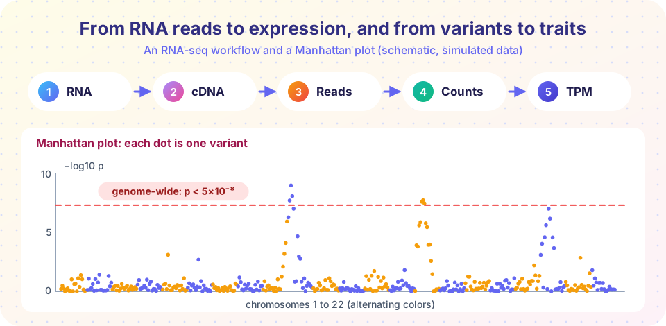
A GWAS compares the genomes of people with a trait (cases) and without it (controls), or measures a quantitative trait such as height or cholesterol, and tests every common variant, typically one to ten million of them, for association. A variant "associated" with disease is one whose allele frequency differs between cases and controls more than chance predicts. The results are displayed as a Manhattan plot: each dot is a variant, the horizontal axis is genome position and the vertical axis is −log₁₀ of the p-value, so the tallest peaks are the strongest signals.
Why the threshold is 5 × 10⁻⁸
If you test one million independent variants and call a result significant at p < 0.05, you would expect about 50,000 false positives by chance alone. A Bonferroni correction divides the threshold by the number of tests. About one million effectively independent common variants exist in people of European ancestry (because variants close to each other are inherited together, called linkage disequilibrium), so 0.05 ÷ 1,000,000 = 5 × 10⁻⁸ became the standard "genome-wide significance" level. A gentler alternative is controlling the false discovery rate (FDR) with the Benjamini-Hochberg procedure, used in RNA-seq.
What GWAS can and cannot say
- Signals point to regions, not to causal genes. Linked variants all show association, and fine-mapping and functional experiments are needed to identify the causal variant.
- Effects of common variants on complex traits are usually small (a few percent change in risk), and many traits are influenced by thousands of variants. Adding them gives a polygenic risk score, which can help stratify risk but is not a diagnosis.
- Association is not causation, and most large GWAS used participants of European ancestry, so scores can be less accurate for other groups, an equity problem researchers are working to fix.
- Single-gene (Mendelian) diseases like cystic fibrosis are better found by family studies and sequencing than by GWAS.
Common misconceptions
"TPM tells you the absolute number of molecules." TPM is a relative measure: the share of the transcript pool, scaled to one million.
"The top GWAS SNP is the disease gene." It marks a region; the causal variant may be a different, linked one.
"A p-value of 0.001 is very strong in a GWAS." With a million tests, thousands of results reach p < 0.001 by chance.
Try it
The first example computes TPM from read counts and gene lengths for five invented genes, and shows how it differs from raw counts and from counts per million.
Press Run (or Ctrl + Enter) to see the result here.
Program input · what you'd type while the program runs
Type the answers before you press Run, one per line. Each time the program reads a line (with input()), it gets the next line from this box.
The second example simulates a Manhattan plot. Most variants are null; three regions carry a planted association. The data are simulated for teaching, and the code draws the genome-wide line at 5 × 10⁻⁸.
Press Run (or Ctrl + Enter) to see the result here.
Program input · what you'd type while the program runs
Type the answers before you press Run, one per line. Each time the program reads a line (with input()), it gets the next line from this box.
The third example demonstrates multiple testing. It tests many null hypotheses, counts false positives at p < 0.05 and at the Bonferroni level, and shows the Benjamini-Hochberg adjustment on a small list of p-values.
Press Run (or Ctrl + Enter) to see the result here.
Program input · what you'd type while the program runs
Type the answers before you press Run, one per line. Each time the program reads a line (with input()), it gets the next line from this box.
Check your understanding
Quick check · 5 questions
of 5 answered You scored / 5 · perfect!
-
1. Why is TPM better than raw read counts for comparing genes within a sample?
Longer genes give more fragments, so counts must be divided by length and scaled to the sequencing depth. -
2. Which type of variant changes a single base?
SNVs/SNPs change one nucleotide; CNVs and translocations are larger structural changes. -
3. A population has allele frequencies p = 0.9 and q = 0.1. Under Hardy-Weinberg, what fraction are heterozygous?
2pq = 2 × 0.9 × 0.1 = 0.18. -
4. The genome-wide significance threshold of 5 × 10⁻⁸ comes from
It is a Bonferroni-style correction for about one million independent common variants. -
5. A strongly associated SNP in a GWAS most likely shows
Linked variants share the signal, so further work is needed to find the causal one.
Summary
- RNA-seq counts reads per gene; TPM normalizes for length and depth so values sum to a million.
- Variants range from single bases to large structural changes and are described by allele frequency; Hardy-Weinberg gives genotype frequencies.
- GWAS tests millions of variants and displays results as a Manhattan plot; the threshold 5 × 10⁻⁸ corrects for multiple testing.
- Signals identify regions, not proven causal genes, and polygenic scores are probabilities, not diagnoses.
Track your progress
Create a free account to tick off lessons and pick up where you left off on any device.
of Molecular Biology lessons completed