


















Lesson 23 of 48 · Climate Records and Proxies
Chapter review: climate records and proxies
Review chapter 4: what thermometers, ice cores, tree rings, corals and sediments measure, how far back they reach, how orbital cycles pace the ice ages, with a ten-question quiz.
Chapter 4 answered the question "how do we know?" You saw that the instrumental record of the last 170 years is built from thousands of stations, ships, floats and satellites that are corrected and cross-checked by independent teams. You saw that ice cores preserve samples of ancient air and the isotopes of ancient snow, that tree rings, corals and ocean sediments extend the record year by year, century by century and across millions of years, and that slow orbital cycles set the rhythm of the ice ages. This review collects the key points and tests them.
What you should be able to do now
- Say what each major archive measures, how it is dated and how far back it reaches.
- Explain homogenization, area weighting and why the urban heat island does not explain global warming.
- Convert isotope shifts to temperature using a calibration slope and explain what ice volume does to foraminifera δ¹⁸O.
- Describe eccentricity, obliquity and precession, and why feedbacks are needed.
- Compare the ice age cycles, the Pliocene and the present in terms of CO₂, temperature and rates of change.
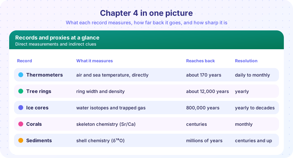
The chapter in a table
| Record | Measures | Reach | Resolution | Main limitation |
|---|---|---|---|---|
| Thermometers and satellites | Air, sea and atmosphere temperature directly | Up to about 170 years (global); some stations since the 1600s | Daily to monthly | Coverage gaps before 1900, instrument changes |
| Tree rings | Ring width and wood density (temperature or moisture) | About 12,000 years | Yearly | Site-specific, age trend, divergence at some sites |
| Corals | Sr/Ca and δ¹⁸O of the skeleton (sea temperature, salinity) | Centuries (fossil corals longer) | Monthly | Local, depends on a few sites |
| Ice cores | Isotopes (temperature), air bubbles (CO₂, CH₄), dust, volcanic sulfate | Up to 800,000 years | Yearly to decades | Gas younger than ice, polar sites only |
| Ocean sediments | Foraminifera shell chemistry (ice volume and temperature) | Millions of years | Centuries to millennia | Bioturbation mixing, coarse dating |
| Cave deposits | Isotopes (rainfall), precise U-Th dates | Hundreds of thousands of years | Yearly to decades | Regional, rainfall mostly |
Connecting the lessons
The chapter's chain of reasoning has four links. First, the instrumental record, assembled from many sources and cross-checked, shows about 1.1 °C of warming and CO₂ rising from about 315 ppm (1958) to over 420 ppm. Second, ice cores show that, for 800,000 years before the industrial era, CO₂ stayed between about 180 and 300 ppm and moved in step with temperature. Third, tree rings, corals and sediments agree on the shape of the last 2,000 years and the larger swings of the ice ages. Fourth, the pace of the ice ages was set by orbital cycles and amplified by feedbacks, in line with the physics of chapter 3.
What ties them together is that independent methods, each with its own uncertainties, give a consistent picture. A single proxy can mislead; several that agree rarely do. That is the logic behind the confidence that the IPCC expresses when it says that recent warming is unusual over at least 2,000 years and that CO₂ is at its highest level in at least 800,000 years of direct ice core data.
Practice: the numbers behind the chapter
The TryIt below collects four calculations from the chapter so you can check your understanding by changing the inputs: an isotope-to-temperature conversion, the CO₂ comparison between ice ages and today, rates of warming and the Nye-model age at depth.
Press Run (or Ctrl + Enter) to see the result here.
Program input · what you'd type while the program runs
Type the answers before you press Run, one per line. Each time the program reads a line (with input()), it gets the next line from this box.
Common misconceptions to leave behind
"Adjusted data are fake data." Adjustments remove known non-climate artifacts, and they are published and tested. They reduce the global warming trend slightly overall.
"The proxies are only guesses." Each proxy rests on a physical or biological process that has been calibrated against measurements and cross-checked with independent archives.
"Ice ages show that climate always changes naturally, so today's change must be natural." Natural changes had causes: orbital cycles and feedbacks. The present change has a measured cause (added greenhouse gases) and is about ten times faster than the last deglaciation.
Worked review problems
Problem 1: reading an ice core. In an Antarctic core the deuterium (δD) value for a layer is 45 ‰ lower than in the Holocene. Using the calibration of 6 ‰ per °C, the local temperature was 45 / 6 = 7.5 °C lower. The global mean change for the same event would be smaller, perhaps around 4 to 5 °C, because polar regions change more than the planet as a whole (polar amplification works in both directions). The result is an estimate for one site; scientists compare it with other cores and proxies.
Problem 2: when does a trend show through the noise? Suppose a proxy record has yearly scatter of 0.4 °C and a real trend of 0.01 °C per year. Over n years the slope uncertainty is about 0.4 / √(n(n² - 1)/12). For n = 50 the sum of squares is 50 × 2499 / 12 = 10,412, so the slope uncertainty is 0.4 / 102 = 0.0039 °C per year, and the trend of 0.01 °C per year is about 2.5 times its uncertainty: detectable. For n = 20 the sum is 665 and the uncertainty is 0.016 °C per year, larger than the trend itself. This is why long records matter and why combining many proxies improves detection.
Problem 3: evaluating a claim. Someone says: "Ice cores show that CO₂ follows temperature, so CO₂ does not affect temperature." Apply the chapter. First, the observation is correct for the start of deglaciations: Antarctic temperature begins to rise a few hundred years before CO₂. Second, the inference does not follow, because a lag does not exclude an effect. In a feedback, a change in one quantity triggers a change in the other, which then pushes back. Third, the physics of chapter 3 says CO₂ absorbs infrared, and the temperature rise after the CO₂ rise is observed in the same ice cores. A careful reply would add that orbital changes start the process, CO₂ amplifies it, and in the modern era CO₂ is rising first because we are adding it.
How to judge a climate claim about the past
The three problems suggest a short checklist for any statement about past climate. First, what is the record: instrumental, or which proxy? Second, how is it dated, and how finely? Third, how was it calibrated and what is the uncertainty? Fourth, do independent records agree? A claim that rests on one record, with no uncertainty, and that contradicts several independent ones should be treated with caution. A claim supported by several independent archives, with stated uncertainties, deserves confidence. Applying this checklist is a habit you can use well beyond this course.
Check your understanding
Quick check · 10 questions
of 10 answered You scored / 10 · perfect!
-
1. Which record can sample ancient atmospheric gases directly?
Bubbles in polar ice trap air from the time the snow became ice. -
2. How do the Sr/Ca ratio and δ¹⁸O in coral relate to temperature?
Both decrease with warming; combining them helps separate temperature from salinity. -
3. Why do ice-age foraminifera shells have higher δ¹⁸O?
Both cooling and ice volume raise shell δ¹⁸O. -
4. How much of the last ice age's global cooling is estimated?
Global cooling at the last glacial maximum was about 6 °C (range 5 to 7). -
5. Which orbital cycle is associated with a period near 41,000 years?
Obliquity (axis tilt) varies between 22.1° and 24.5° with a 41,000-year period. -
6. Why are feedbacks needed to explain ice ages?
The orbital push is strong in some regions and seasons but weak globally; ice-albedo and CO₂ feedbacks amplify it. -
7. How do the 'CO₂ lags temperature' findings fit with greenhouse physics?
Orbital changes start the warming, CO₂ rises later, and then adds to the warming. -
8. A 2.4 °C urban excess over 3 % of the land surface (29 % of the globe) would change the global mean by about 0.02 °C. What does this suggest?
Because cities cover so little of the planet, even a large local excess hardly moves the global mean. -
9. Which statement about the IPCC's conclusion on the past is correct?
Multi-proxy reconstructions and instrumental data support this finding. -
10. About how much faster is the present rate of warming than the average rate during the last deglaciation?
About 0.65 °C per century since 1850 versus about 0.06 to 0.1 °C per century at the end of the last ice age.
Summary
- The instrumental record, combined from stations, ships, floats and satellites and cross-checked by independent groups, shows about 1.1 °C of warming since 1850-1900.
- Ice cores give 800,000 years of CO₂ (180 to 300 ppm), methane and isotopic temperature; tree rings, corals and sediments extend and cross-check the record.
- Orbital cycles (100,000/400,000, 41,000 and 19,000 to 23,000 years) set the ice-age rhythm, with feedbacks amplifying the effect.
- Independent archives agree, and recent warming is unusual in at least 2,000 years and about ten times faster than the last deglaciation.
- Chapter 5 now shows how climate models use this physics to project the future.
Track your progress
Create a free account to tick off lessons and pick up where you left off on any device.
of Climate Science lessons completed