


















Lesson 44 of 48 · Projects and Practice
Project: a two-box climate model
Code a two-box climate model with a fast surface layer and slow deep ocean, then measure equilibrium and transient sensitivity and explore committed warming.
In Chapter 5 you met the one-box energy balance model, C dT/dt = F − λT. It captures the idea of equilibrium sensitivity, but it has a flaw: it predicts that the climate responds to a forcing with a single time constant of a few years. The real climate shows both a quick response (the surface and upper ocean warm within years) and a slow one (the deep ocean keeps absorbing heat for centuries). Adding a second box for the deep ocean fixes this, and with a dozen lines of Python you can reproduce features that big models show: the gap between transient and equilibrium warming, and warming that continues after forcing stops rising.
This project walks you through building the model, testing it, measuring its sensitivity, and exploring "committed warming." You will work with numbers close to those used in simple climate emulators in research.
What you will learn
- Translate coupled differential equations into a numerical simulation.
- Test a model against a known analytic result.
- Measure equilibrium and transient climate response in the model.
- Explain committed warming and why ocean heat uptake delays the response.
The equations
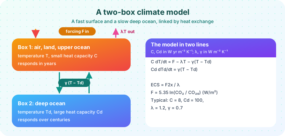
Let T be the temperature change of the upper box (air, land and the ocean mixed layer) and T_d that of the deep ocean, both relative to the preindustrial state. The model is:
C  dT/dt   = F(t) − λ T − γ (T − T_d)
C_d dT_d/dt = γ (T − T_d)
F(t)is the radiative forcing in W/m². For CO₂ we useF = 5.35 ln(CO₂ / CO₂₀), so a doubling givesF₂ₓ = 5.35 ln 2 = 3.71 W/m².λis the climate feedback parameter, W m⁻² K⁻¹. The equilibrium sensitivity isECS = F₂ₓ / λ.γis the heat exchange coefficient between the boxes, W m⁻² K⁻¹.CandC_dare heat capacities in W yr m⁻² K⁻¹. The upper box is small (the ocean mixed layer plus land and air, about 8) and the deep ocean is large (about 100 in effective terms).
We use illustrative values C = 8, C_d = 100, λ = 1.2, γ = 0.7. With these, ECS = 3.71 / 1.2 ≈ 3.1 °C, similar to the IPCC's best estimate. Real two-box fits to climate models use values in this neighborhood, but treat the numbers as a teaching set, not a calibrated model.
Units check. C dT/dt has units (W yr m⁻² K⁻¹)(K yr⁻¹) = W m⁻². That matches λT (W m⁻² K⁻¹ × K). Always verify that every term in an equation has the same units.
Step 1: simulate and test
We step the equations forward with the Euler method: T(t + Δt) = T(t) + Δt × (dT/dt). With a time step of 0.1 year it is accurate enough here (the fastest time constant is about C/(λ+γ) ≈ 4 years, far longer than 0.1). A good test: hold the forcing constant at F₂ₓ. Eventually both boxes should settle at T = T_d = F₂ₓ/λ, the equilibrium. In the simulation that takes many centuries, because of the large deep box. Test with 1,500 years and print the result.
Press Run (or Ctrl + Enter) to see the result here.
Program input · what you'd type while the program runs
Type the answers before you press Run, one per line. Each time the program reads a line (with input()), it gets the next line from this box.
You should see the upper box reach more than half of its eventual value within a decade and about two thirds within a few decades, then creep up slowly as the deep ocean warms. This two-timescale behavior is not possible in a one-box model.
Step 2: transient and equilibrium response
The transient climate response (TCR) is the warming at the time CO₂ doubles when it rises by 1% per year. Doubling takes ln 2 / ln 1.01 ≈ 70 years. The forcing in that experiment is F(t) = 5.35 ln(1.01^t) = 5.35 t ln 1.01. Run it and read the upper-box temperature at year 70. Compare with the equilibrium sensitivity: the ratio TCR/ECS tells you how much warming is "hidden" by ocean heat uptake. The IPCC assessed TCR as 1.8 °C (likely 1.4 to 2.2 °C) against an ECS of 3 °C, so a ratio of about 0.6 is realistic.
Press Run (or Ctrl + Enter) to see the result here.
Program input · what you'd type while the program runs
Type the answers before you press Run, one per line. Each time the program reads a line (with input()), it gets the next line from this box.
Step 3: committed warming
Here is the most important experiment. Increase CO₂ by 1% per year until it doubles at year 70. Then hold the CO₂ concentration constant, so the forcing stays at F₂ₓ. Does the temperature stop rising? No. The deep ocean is still far cooler than the surface, so heat keeps flowing downward, but as it does the upper box also keeps adjusting to the constant forcing and warms further. The extra warming after year 70 is the committed warming from the concentrations already reached.
Many people imagine that stopping rising CO₂ concentration would stop warming. The model shows otherwise (the real world is similar, with studies of "zero emissions commitment" being more subtle because stopping emissions also lets sinks pull CO₂ down).
Press Run (or Ctrl + Enter) to see the result here.
Program input · what you'd type while the program runs
Type the answers before you press Run, one per line. Each time the program reads a line (with input()), it gets the next line from this box.
Why two boxes are better than one
Compare the model with the single-box equation from Chapter 5. A one-box model with C = 8 has one time constant of about six years, so it says that the climate reaches nearly full equilibrium within a few decades. The two-box model reproduces the observation that part of the response is quick and part is slow, and it gives a TCR noticeably below ECS, as seen in comprehensive models and in the observed record. It does so with only two extra parameters. This is the spirit of simple models in climate science: add the minimum ingredient that explains a feature of the data or of a complex model, and no more. Researchers use two- and three-box fits as emulators, quick stand-ins that reproduce a big model's global-mean response so that thousands of scenarios can be explored. A good emulator is tested against the big model it imitates, and its parameters are chosen to match several features at once.
Reading your results
- Step 1 confirms the code against theory (equilibrium
F/λ). A model that fails such a test should not be trusted. - Step 2 gives a TCR below the ECS. The gap is the heat taken up by the deep ocean. Make
γlarger and the TCR falls (more heat is hidden), makeγzero and the model collapses to one box, with TCR close to ECS. - Step 3 shows committed warming: some warming is "in the pipeline" even if concentrations are held fixed. If emissions instead drop to zero, CO₂ also declines slowly as the ocean and land absorb it, and the two effects roughly cancel, which is why many studies find little further warming after net zero.
Experiments to try
- Feedback strength. Change
λto 0.9 and 1.8. How do TCR and ECS change? - Ocean uptake. Change
γto 0.3, 0.7 and 1.2. Which temperature responds most in the first 70 years? - Emissions to forcing. Replace the forcing with a smooth curve that rises, peaks and then falls (a peaking scenario). When does the upper box peak compared with the forcing?
- Heat capacity. Double
C_d. How much longer does the system take to get close to equilibrium? - Compare with the one-box model. Set
γ = 0and compare the temperature at year 70.
What this model leaves out. It uses a constant feedback parameter (real feedbacks vary with the state of the climate and the pattern of warming), represents the ocean as a single deep reservoir, includes no carbon cycle and no regional detail. It is a useful emulator of the global mean, and a poor guide to local climate.
Check your understanding
Quick check · 5 questions
of 5 answered You scored / 5 · perfect!
-
1. In the two-box model, what is the equilibrium warming for constant forcing F?
At equilibrium T = T_d and the heat exchange term vanishes, leaving F = λT. -
2. Why is the transient climate response lower than the equilibrium sensitivity?
Heat uptake by the deep ocean delays the surface response. -
3. What happens after concentrations stop rising in the model?
The system has not reached equilibrium, so committed warming remains. -
4. What does the Euler method do?
It updates each variable by its rate of change times the time step. -
5. If γ is set to zero, the model reduces to
Without heat exchange the upper box is isolated, giving the simple energy balance model.
Summary
- The two-box model has a fast upper box and a slow deep ocean linked by heat exchange.
- Equilibrium warming is
F/λ; transient warming is lower because of ocean heat uptake. - A numerical simulation must be tested against known results such as the equilibrium.
- Warming continues after concentrations stop rising: that is committed warming.
- Simple emulators are valuable for global-mean questions but leave out much of the real system.
Next: Practice problems
Track your progress
Create a free account to tick off lessons and pick up where you left off on any device.
of Climate Science lessons completed