


















Lesson 43 of 48 · Projects and Practice
Project: an emissions pathway calculator
Build a small Python tool that turns an emissions pathway into cumulative CO2, a carbon budget check and implied warming, then explore how delay changes the cuts needed.
In this project you will build a small tool that does what climate analysts do all the time: take an emissions pathway, a curve showing how annual CO₂ emissions change over the coming decades, and ask what it implies. Does it stay within a carbon budget? How much warming does it add? What happens if we wait ten years before starting to cut?
You will write the code in steps, test each piece against hand calculations from Chapter 7, and finish with experiments. Along the way you practice a skill that matters in any quantitative science: building a simple model, checking it, and being honest about what it leaves out.
What you will learn
- Represent emission pathways as functions of time.
- Compute cumulative emissions and compare them with a carbon budget.
- Convert cumulative CO₂ into implied warming using TCRE.
- Solve for the latest start year that still meets a budget.
- State the limits of a simple model.
The model in one page
The project uses four ideas you already know.
- Annual emissions
E(t)in gigatonnes of CO₂ per year. We start fromE₀ ≈ 37 Gtof fossil CO₂ in 2025 (a round number; land use adds a few Gt more). - Cumulative emissions
C = Σ E(t), the sum over years. This is the area under the pathway. - A carbon budget
Bin Gt CO₂, such as the 500 Gt for a 50% chance of 1.5 °C counted from 2020. By 2025 several years of emissions have used part of it, which is why we later try budgets of different sizes. - Implied warming
ΔT ≈ ΔT_now + TCRE × C, withTCRE = 0.45 °C per 1000 Gtand today's warming about 1.2 °C.
We only model CO₂ and ignore other gases, aerosols, the exact Earth-system response and negative emissions. Those omissions matter for real budgets (they shift the numbers by tens of percent), so you should treat the results as lessons, not forecasts.
Modeling habit: write down the assumptions before you code. Here: constant start emissions, a straight-line decline, CO₂ only, warming proportional to cumulative emissions. If any assumption is wrong for your question, the answer is too.
Step 1: pathways as functions
A pathway needs a start year, a year when cuts begin, and a year when emissions reach zero. Before the cut year emissions stay constant; afterward they fall in a straight line. Write it so it works for any numbers, and test it on a case you can check by hand: start at 40 Gt, cut from 2025, zero in 2065 (40 years). The cumulative total is a triangle: ½ × 40 × 40 = 800 Gt.
Press Run (or Ctrl + Enter) to see the result here.
Program input · what you'd type while the program runs
Type the answers before you press Run, one per line. Each time the program reads a line (with input()), it gets the next line from this box.
The small difference between the simulated sum and 800 is a discretization effect: a sum of yearly values vs the area of a triangle. If you wanted more accuracy you could use half-weights at the ends (the trapezoid rule). For this project the difference is far below the uncertainty in the budget.
Step 2: budgets and warming
Now add a function that converts cumulative emissions into implied warming and compares them with a budget. Then run four policies:
- Early and steady: start cutting in 2025, zero in 2050.
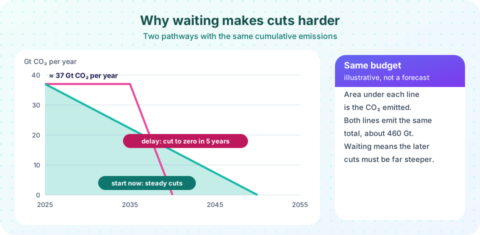
- Delayed: keep emissions flat until 2035, then cut to zero in 2055.
- Slow: start in 2025 but take until 2080 to reach zero.
- No policy: emissions flat forever (we cut off the run in 2100).
Plot them and print the cumulative total, the budget check and implied warming.
Press Run (or Ctrl + Enter) to see the result here.
Program input · what you'd type while the program runs
Type the answers before you press Run, one per line. Each time the program reads a line (with input()), it gets the next line from this box.
You should see that only the early, steady pathway is anywhere near the budget, and that the slow pathway overshoots despite starting right away. The area, not the start date alone, decides.
Step 3: how long can we wait?
A useful question for policy: given a budget and a target year for zero, what is the latest year we can start cutting? Rather than doing algebra, you can scan over start years and find the last one that fits. That is a pattern worth knowing: when a formula is messy, sweep a parameter and look for the boundary.
Press Run (or Ctrl + Enter) to see the result here.
Program input · what you'd type while the program runs
Type the answers before you press Run, one per line. Each time the program reads a line (with input()), it gets the next line from this box.
Notice the "impossible" entries: with a small budget, even starting today and cutting in a straight line to a late zero emits too much. That is exactly what the IPCC's finding about steep, immediate cuts for 1.5 °C means.
Reading your results
Compare your results with what you know.
- With
B = 500andzero_year = 2050, the latest start year should be close to the present. The reason is that a straight line from 37 Gt to zero over 25 years emits½ × 37 × 25 ≈ 460 Gt, nearly the whole budget. - A budget of 900 Gt allows later starts or a later zero year, which is why the probability level and temperature target matter so much for how urgent action seems.
- The implied warming for the "no policy" path is large because the total in 75 years at constant emissions is about 2,800 Gt, giving
1.2 + 0.45 × 2.775 ≈ 2.5 °C. A real no-policy world would also have growing or shrinking emissions, which is why scenarios exist.
Checking your own work
A good model has checks. Try these:
- Set
E0 = 0: every result should be zero. - Set
cut_year = zero_year - 1: the pathway is almost a step function; the cumulative total should be close toE0 × (cut_year - 2025). - Double
E0and halveTCRE: the warming should not change (it depends only on the product).
If any check fails, you have a bug, and finding it will teach you something about your code.
Interpreting the results as a decision-maker
Imagine you are advising a government. The calculator tells a clear story, but a decision-maker needs the story in plain language. First, the budget is a constraint on the total, so a target year is only meaningful together with the path to it. Second, the cost of delay is not linear: each year of waiting removes budget and adds steepness, so the required annual cut rate rises faster and faster. Third, the answer depends on the budget you choose, which depends on the temperature goal, the probability of success and how non-CO₂ gases are treated. A fair presentation shows several budgets side by side instead of one number. Finally, the model says nothing about how to achieve the cuts or what they cost. For that you need the mitigation toolbox from Chapter 7 and the policy tools from Chapter 8. Practice writing a three-sentence summary of your results for a non-specialist, then check that each sentence can be traced to a line of output.
Extensions
Pick one or two to try.
- Exponential decline. Replace the straight line with
E(t) = E₀ e^(−r (t − t_cut))and find the rate that exactly uses the budget. - Non-CO₂ gases. Add a flat 0.1 °C of extra warming for methane, or shrink the budget by 10%.
- Negative emissions. Let emissions go negative after net zero (removals) and see how it changes the late-century warming.
- Uncertainty. Run the model with
TCREdrawn from a range of 0.27 to 0.63 °C per 1000 Gt and show a band of outcomes. - Regional view. Split
E0between two regions with different cut times and see how fairness and timing interact.
Limits of the model. It treats emissions as a smooth curve, ignores the carbon already spent since the budget was defined, ignores non-CO₂ gases and aerosol cooling, and assumes TCRE is constant. Real budgets come from Earth system models and carry uncertainty of at least a few hundred Gt. Always say which assumptions your result depends on.
Check your understanding
Quick check · 5 questions
of 5 answered You scored / 5 · perfect!
-
1. What does the area under an emissions pathway represent?
Summing annual emissions over time gives the cumulative total. -
2. A pathway falls linearly from 40 Gt per year to zero over 25 years. The cumulative total is about
The area of the triangle is ½ × 40 × 25 = 500 Gt. -
3. Why does delaying cuts by ten years force steeper cuts later, for the same budget?
More budget is used before cuts start, leaving less for the remaining years. -
4. What does the scanning approach in Step 3 do?
Sweeping a parameter is a robust way to find a boundary when algebra is awkward. -
5. Which assumption does this model make?
The model uses TCRE to convert cumulative CO₂ to warming and ignores other gases.
Summary
- A pathway is a function of time; cumulative emissions are the area under it.
- Comparing the area with a budget, and multiplying by TCRE, turns a pathway into implied warming.
- Delay shrinks the remaining time, so later cuts must be much steeper.
- Sweeping a parameter finds the latest start year without algebra.
- Always check a model against hand calculations and state its limits.
Track your progress
Create a free account to tick off lessons and pick up where you left off on any device.
of Climate Science lessons completed