


















Lesson 3 of 48 · Getting Started
Anomalies, baselines and trends
Learn why climate scientists plot temperature anomalies instead of raw temperatures, how a baseline is chosen, and how to measure a trend with a least-squares line.
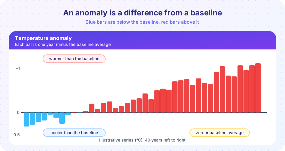
Open any chart of global warming and you will almost certainly see a vertical axis labeled "temperature anomaly" rather than "temperature". The reason is practical, not mysterious. A thermometer on a mountain and a thermometer on a beach will never agree in absolute terms, yet both can tell you perfectly well whether this year was warmer than usual. Anomalies are the tool that turns thousands of mismatched thermometers into one coherent picture.
In this lesson you learn what an anomaly is, how the baseline behind it is chosen, why changing the baseline never changes the trend, and how to measure a trend with a straight-line fit. These skills carry through the whole course: nearly every climate chart you meet is an anomaly chart.
What you will learn
- Define an anomaly and compute one from a baseline.
- Explain why anomalies are better than raw temperatures for combining stations.
- Name the common baseline periods and say why changing the baseline shifts but does not tilt a series.
- Fit a trend line and interpret its slope in degrees per decade.
- Recognize when a short trend is unreliable.
Key terms
Anomaly: the difference between a measurement and the average of a reference (baseline) period. Baseline: the reference period whose average defines zero, such as 1951 to 1980. Trend: the average rate of change of a series, usually the slope of a least-squares line. Least squares: a method that picks the line minimizing the sum of squared vertical distances to the data. Pre-industrial: a reference of roughly 1850 to 1900, before large-scale fossil-fuel burning.
Why raw temperatures mislead
Suppose two weather stations sit 40 km apart. One is in a valley at 50 m elevation and averages 12 °C in a year. The other is on a ridge at 900 m and averages 6 °C. Temperature falls roughly 6.5 °C for each kilometer you climb, so the 6-degree gap is entirely expected. If you averaged the two readings you would get 9 °C, a number that describes neither place. Worse, if the ridge station is closed for a year, the combined average suddenly jumps by 3 °C although nothing happened to the climate.
The fix is to subtract each station's own normal from its own readings first. Now the valley and ridge both report the difference from their own usual conditions. If July is 1 °C warmer than normal in the valley and 0.9 °C warmer on the ridge, both stations tell the same story, and you can average them safely. Anomalies are also strongly correlated over large distances. Work by James Hansen and Sergej Lebedeff in 1987 showed that anomalies at stations correlate over roughly 1,000 km, whereas absolute temperatures differ wildly over a few tens of kilometers. This allows a sparse network to represent the globe sensibly.
How to compute an anomaly
The recipe has three steps.
- Choose a baseline period (for example, 1991 to 2020).
- For each station and each calendar month, average the baseline years to get the normal.
- For every measurement, subtract the normal for that station and month.
Subtracting the normal per calendar month removes the seasonal cycle, so an anomaly for January and an anomaly for July are comparable. Global anomalies are then averaged over a grid of the Earth's surface, weighting each cell by its area.
Worked example
A station's July highs over a 30-year baseline average 17.2 °C. This July the monthly mean high was 18.1 °C. The anomaly is 18.1 - 17.2 = +0.9 °C. In the same year the January normal is 2.0 °C and the January value was 1.4 °C, an anomaly of -0.6 °C. Note that July is 16 degrees warmer than January in absolute terms, yet both anomalies are small numbers of the same kind, which is exactly why they can be combined into one yearly series.
Choosing the baseline
Different agencies use different baselines, so the same warming appears with different numbers.
| Source or purpose | Typical baseline |
|---|---|
| NASA GISTEMP | 1951 to 1980 |
| HadCRUT (UK Met Office and University of East Anglia) | 1961 to 1990 |
| WMO current climate normal; Copernicus reanalysis | 1991 to 2020 |
| IPCC warming reports and the Paris Agreement targets | 1850 to 1900 (pre-industrial) |
None of these is the "right" one; each is a choice made for a purpose. A recent baseline gives a stable, well-measured average. A pre-industrial baseline answers the question that policy cares about: how far above the world before industrialization are we? Because earlier thermometer coverage is sparse, the pre-industrial average is estimated with more uncertainty.
Changing the baseline
Switching baseline subtracts a different constant from every value. The entire series slides up or down together, but the differences between years, and therefore the slope, stay exactly the same. A trend of 0.2 °C per decade is 0.2 °C per decade whether zero is 1951 to 1980 or 1991 to 2020. When two charts appear to disagree about "how much warming", check the baselines before suspecting the data.
What about the absolute global temperature?
Climate scientists do estimate the absolute global mean surface temperature. It is about 14 °C for the second half of the twentieth century, but the figure is known less precisely (by roughly half a degree) than the anomaly is. That is not a flaw: anomalies are known well because the baseline cancels many local biases, while an absolute average depends on how well mountains, polar regions and oceans are sampled.
Measuring a trend
A trend is the average rate of change. The simplest way is the least-squares line through the points. Its slope is the trend, typically quoted in degrees per decade. For n data points (x, y) the slope is
slope = Σ(x - x̄)(y - ȳ) / Σ(x - x̄)²
and the line passes through the point of averages. Spreadsheets, NumPy's polyfit and every statistics package compute it.
Beware short records
A short window can mislead. If yearly noise is about 0.15 °C, the slope of a 10-year trend has a standard deviation of about 0.17 °C per decade by chance alone, so even steady warming of 0.2 °C per decade occasionally appears as a "pause" in a ten-year slice (the second TryIt shows how often). To read a trend honestly you ask how large the uncertainty on the slope is, which depends on the noise and the length of the record. Longer windows, or combining several independent datasets, give much tighter answers.
Common misconceptions
"Anomalies hide the real temperature, so they must be manipulated." An anomaly is just a subtraction, and any reader can reverse it by adding the baseline back. It is used because it removes sampling bias between stations, not to conceal anything.
"Different organizations show different warming, so the science is uncertain." Different baselines shift charts up or down. The year-to-year changes and the long-term slope agree closely among independent datasets, as chapter 4 shows.
"Ten years without a record means warming stopped." Ten-year windows are dominated by noise such as El Niño and La Niña. A trend must be judged over a longer period, with an uncertainty range.
Try it
The first example creates two invented stations with different mean temperatures but the same warming. Raw values disagree; anomalies agree.
Press Run (or Ctrl + Enter) to see the result here.
Program input · what you'd type while the program runs
Type the answers before you press Run, one per line. Each time the program reads a line (with input()), it gets the next line from this box.
The second example fits a trend and shows how a short window can mislead. The data are simulated with a true trend of 0.2 °C per decade.
Press Run (or Ctrl + Enter) to see the result here.
Program input · what you'd type while the program runs
Type the answers before you press Run, one per line. Each time the program reads a line (with input()), it gets the next line from this box.
The third example is a baseline slider: it moves the zero line and shows that the trend (the slope of the red line) does not change.
Check your understanding
Quick check · 5 questions
of 5 answered You scored / 5 · perfect!
-
1. A station has a July normal of 20.0 °C. This July it recorded 21.5 °C. What is the anomaly?
Anomaly equals measurement minus normal: 21.5 - 20.0 = +1.5 °C. -
2. Why are anomalies better than raw temperatures for combining stations at different elevations?
Subtracting each station's own normal removes site-specific offsets, leaving changes that are comparable across places. -
3. What happens to the trend when you switch the baseline from 1951-1980 to 1991-2020?
Changing the baseline subtracts one constant from every value, which moves the series but does not change differences between years. -
4. Which baseline is closest to the 'pre-industrial' reference used for Paris Agreement targets?
The IPCC and the Paris Agreement use roughly 1850 to 1900 as the reference for global warming. -
5. Why can a 10-year trend be misleading?
With noise of the size of year-to-year variability, a short window can show a slope very different from the long-term trend.
Summary
- An anomaly is a value minus the average of a baseline period; it removes site-specific offsets and the seasonal cycle.
- Anomalies are correlated over large distances, so they can be combined into regional and global averages.
- Baselines differ among datasets (1951-1980, 1961-1990, 1991-2020, 1850-1900) but changing one only shifts the series.
- A trend is the least-squares slope, usually in degrees per decade; short windows carry large uncertainty.
- Compare charts only after checking their baselines.
Track your progress
Create a free account to tick off lessons and pick up where you left off on any device.
of Climate Science lessons completed