


















Lesson 5 of 48 · Getting Started
Chapter review: Getting Started
Review chapter 1 of the climate science course with a one-page picture, a recap table, a practice calculation and a ten-question quiz on weather, climate, anomalies and history.
You have now covered the foundation of the whole subject. Chapter 1 gave you three tools that you will use constantly: the distinction between weather and climate, the habit of looking at anomalies and trends, and a sense of how the science grew from nineteenth-century laboratories to a worldwide assessment process. This review pulls them together, gives you one more calculation to try and finishes with a longer quiz.
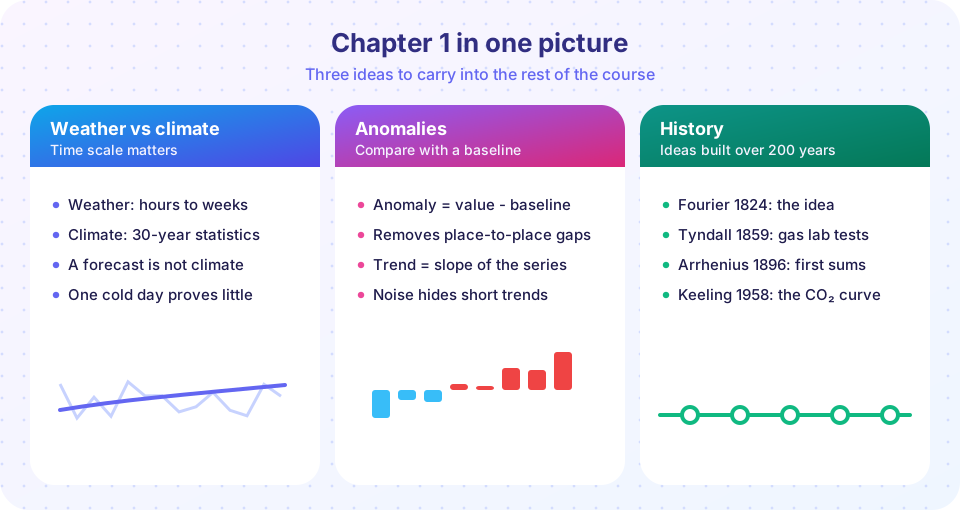
What you should be able to do now
- Say whether a statement describes weather or climate, and explain your choice in terms of time scale.
- Explain why averaging over many years reveals a trend that single years hide, and estimate how much.
- Compute an anomaly from a baseline, and explain why changing the baseline does not change the trend.
- Fit a straight line to a series and read off its slope.
- Name five or six milestones in the history of climate science and what each added.
The chapter in a table
| Idea | One-sentence summary | Where to use it |
|---|---|---|
| Weather | The state of the atmosphere over hours to weeks | Forecasts, daily life |
| Climate | The statistics of weather over about 30 years or more | Planning, climate change |
| Climate normal | A 30-year average used as a reference (now 1991 to 2020) | Defining "typical" |
| Natural variability | Year-to-year ups and downs that are not a long-term trend | Reading short records |
| Signal and noise | A slow change hidden by random scatter | Deciding what a trend means |
| Square-root law | Scatter of an average of n values falls as σ / √n |
Planning how much data is enough |
| Anomaly | Value minus baseline average | Combining stations, plotting warming |
| Baseline | The reference period that defines zero | Comparing charts |
| Trend | Least-squares slope, usually in °C per decade | Measuring change |
| Pre-industrial | About 1850 to 1900, the policy reference for warming | Paris Agreement targets |
Connecting the ideas
The three lessons fit together like parts of a single method. Climate is a statement about statistics, so to detect change you need many observations. Those observations come from instruments that differ in place and quality, so you convert them to anomalies, which can be combined. Even then the combined series is noisy, so you fit a trend and quote its uncertainty, while remembering that short windows mislead.
History adds a reminder about how knowledge is built. Tyndall's laboratory measurement (1859) and Arrhenius's calculation (1896) concern simple physics; Keeling's 1958 record shows that the gas is really increasing; the first models (1967 and 1979) combine the two into a prediction. That chain, where physics gives an expectation, measurements test it and models extend it, will be the pattern for every chapter that follows.
Practice with your own numbers
The TryIt below is a small tool you can reuse. Paste a series of yearly values (for example, annual average temperature at a place you know), choose a baseline, and it prints the anomalies, the trend and a rough uncertainty. The starter data are invented. Replace them with real numbers if you like. Try shortening the window to see how the uncertainty grows.
Press Run (or Ctrl + Enter) to see the result here.
Program input · what you'd type while the program runs
Type the answers before you press Run, one per line. Each time the program reads a line (with input()), it gets the next line from this box.
Common misconceptions to leave behind
"If the trend over 10 years is flat, the long-term trend must have changed." Short windows are noisy. Ask for the uncertainty and for a longer record.
"Anomalies and baselines are a trick to make warming look bigger." Changing the baseline never changes the slope. It changes only where zero sits.
"The history shows scientists keep changing their minds." The central estimate for climate sensitivity has stayed near 3 °C per doubling of CO₂ since 1979; what improved is the confidence.
Worked review problems
Working a few problems by hand is the best way to check that the chapter has stuck. Here are three, with full reasoning.
Problem 1: weather or climate? A newspaper writes: "Last Tuesday was the coldest day of the year in the city, so the climate is not warming." Which two time scales are being confused? The statement uses a single day (weather) to make a claim about a trend over decades (climate). A sound reply would ask for the long-term record: how have the yearly averages and the frequency of cold days changed over the last 30 or 50 years? One day in the cold tail of the distribution is expected to occur occasionally even when the whole distribution is shifting upward, so the observation is consistent with warming and says very little about it.
Problem 2: how much data do I need? A coastal weather station has yearly mean temperatures with random scatter of 0.5 °C around a steady trend of 0.02 °C per year. You want the mean to be reliable to within 0.1 °C (one standard error). The scatter of a mean of n values is 0.5 / √n, so you need √n ≥ 5, that is n ≥ 25 years, ignoring the trend. For a trend measurement you need still more care: the standard error of a slope over n yearly points is σ / √Σ(x - x̄)², and for n = 20 the sum of squares is n(n² - 1)/12 = 665, so the slope uncertainty is 0.5 / 25.8 = 0.019 °C per year. That is almost as large as the true trend of 0.02 °C per year, which is why twenty years of a single noisy station is not enough to establish a trend with confidence. Combining many stations (which reduces the noise) or lengthening the record is the fix.
Problem 3: changing the baseline. A series of anomalies relative to 1951-1980 reads +0.60 °C for the year 2000. The 1991-2020 average of the same series, on the 1951-1980 baseline, is +0.55 °C. What is the year 2000 anomaly relative to 1991-2020? Subtract the new baseline from the old anomaly: 0.60 - 0.55 = +0.05 °C. The shape of the series, and every difference between two years, is unchanged. This is the arithmetic behind the statement that changing the baseline never changes the trend.
How to keep studying
Chapter 1 gave you the habits of mind that scientists use before they start any calculation: ask what the time scale is, ask what is being compared with what, and ask how big the uncertainty is. Keep them in mind as you move on. In chapter 2 you will meet the physical system that produces the numbers you now know how to read. In chapter 3 you will see why temperatures are what they are. In chapter 4 you will return to the records in this chapter and see where they come from.
If any of the review problems felt hard, go back to the matching lesson and rerun its TryIt with different numbers. Changing a single value and predicting the result before you press Run is the fastest way to turn a formula into an intuition. A good target before you move on: explain, without notes, why one cold winter does not say anything about climate, why anomalies are used, and what the Keeling curve measures.
Check your understanding
Quick check · 10 questions
of 10 answered You scored / 10 · perfect!
-
1. The statement 'July in Madrid is usually hot and dry' describes:
It describes what is typical over many years, which is climate. -
2. Yearly values scatter with a standard deviation of 0.5 °C. About how much does a 25-year average scatter by chance?
0.5 / √25 = 0.5 / 5 = 0.1 °C. -
3. Why does a climate normal use about 30 years?
30 years is a convention that balances smoothing against relevance. -
4. A station's baseline mean for March is 8.0 °C. This March it measured 6.7 °C. What is the anomaly?
6.7 - 8.0 = -1.3 °C. -
5. You switch the baseline from 1951-1980 to 1991-2020. What happens to every anomaly in the series?
A different baseline subtracts a different single number from every value. -
6. Which pairing of scientist and contribution is correct?
Keeling measured CO₂ at Mauna Loa and Arrhenius calculated warming in 1896; the IPCC was created in 1988 by the WMO and UNEP. -
7. Which of the following is a reason NOT to base conclusions on a single cold winter?
Single winters are weather; cold spells are still possible in a warming climate. -
8. Which baseline is typically used to define 'pre-industrial' for policy targets?
The IPCC and Paris Agreement refer to about 1850 to 1900. -
9. Why were Ångström's 1900 'saturation' objections eventually answered?
Better spectroscopy and atmospheric physics showed that more CO₂ raises the layer from which heat escapes, even where lower air is already opaque. -
10. A 10-year window shows no warming trend. What is the best response?
With natural variability of the size seen year to year, short slopes have large uncertainty.
Summary
- Climate is the statistics of weather; single events are weather.
- Averaging
nvalues reduces random scatter by√n, and trends need long records. - Anomalies remove site-specific differences; baselines shift series without changing trends.
- The central physics was established between 1824 and 1967, and the IPCC has assessed it since 1988.
- Chapter 2 now opens up the climate system itself.
Track your progress
Create a free account to tick off lessons and pick up where you left off on any device.
of Climate Science lessons completed