


















Lesson 19 of 48 · Climate Records and Proxies
The instrumental record
Learn how global temperature is measured and combined from stations, ships, buoys and satellites, how data are corrected, what the urban heat island does, and what the Keeling curve shows.
The most direct evidence that the climate is changing comes from the most straightforward tools: thermometers, rain gauges and, in the last decades, satellites. Together they produce the instrumental record. It is a global patchwork stitched together from weather stations on land, ships and buoys at sea, balloons in the air and instruments in orbit, and every part of the process (collecting, correcting, combining) has been scrutinized by independent teams around the world.
This lesson explains how the patchwork is built, why raw readings cannot simply be averaged, how scientists handle errors such as station moves and urban growth, and how four independent groups arrive at almost the same answer. It ends with the CO₂ record that Charles Keeling began in 1958.
What you will learn
- Describe the main sources of instrumental data: stations, ships, buoys and Argo floats, satellites.
- Explain why scientists adjust (homogenize) records and how they check the adjustments.
- Explain how a global mean is built from a gridded anomaly field with area weighting.
- Assess the urban heat island objection with numbers.
- Interpret the Keeling curve, including its seasonal cycle.
Key terms
Homogenization: correcting a record for non-climate changes such as moving a station or changing an instrument. Urban heat island (UHI): the extra warmth of cities compared with their surroundings. Reanalysis: a weather model that is run over past decades while assimilating all available observations. Argo: a network of about 4,000 free-drifting floats that measure temperature and salinity in the upper 2,000 m of the ocean. Reference period: the baseline used for anomalies (chapter 1).
Where the data come from
Weather stations on land. Reliable thermometers exist from about the 17th century: the Central England record begins in 1659. Today the Global Historical Climatology Network includes tens of thousands of stations, though only a few thousand have long, continuous records. Standard practice, introduced in the 19th century, is to place the thermometer in a white, ventilated box (a Stevenson screen) about 1.5 m above grass, away from buildings.
Sea surface temperature. The oceans cover 71 % of Earth, so ships have been central. For decades sailors hauled up buckets of water and measured them with thermometers (the water cools in a wooden bucket more than in an insulated one); later, thermometers in engine intakes warmed the readings. Since the 1980s moored and drifting buoys have supplied cleaner measurements. Scientists correct for these changes in method.
The ocean interior. Since about 2000, the Argo array of roughly 4,000 floats has profiled temperature and salinity to 2,000 m every ten days, producing the first truly global record of ocean heat content.
Satellites. From 1979 microwave sounding units on weather satellites measure the temperature of broad layers of the atmosphere from the radiation emitted by oxygen. Other satellites track sea ice area, sea level (radar altimeters, since 1993), and the energy that Earth absorbs and emits (the CERES instruments, since 2000). These records need careful corrections for orbit drift and sensor changes, and early disagreements between different teams were largely resolved by finding and fixing such errors.
Why we use anomalies and grids
A global mean cannot be computed by averaging raw station values, for the reasons in chapter 1. Instead, scientists compute an anomaly for each station and month, average anomalies within boxes on a latitude-longitude grid (typically 2° to 5°), and then combine the boxes with weights proportional to area. The area weighting matters: boxes near the poles are narrow, and the area of a box scales with the cosine of its latitude. An unweighted average would give polar boxes, where warming is fastest and data are sparse, far too much influence.
Making the record homogeneous
Raw records contain non-climate jumps. A station may be moved from a city center to an airport. A mercury thermometer may be replaced by an electronic sensor. The time of day when the observer reads the thermometer may change, which shifts daily averages. Left alone, these would look like steps in temperature.
Homogenization compares each station's series with those of its neighbors, which share the same weather. If one station suddenly warms or cools by 0.5 °C relative to all the others in a given year, it is likely that something non-climatic happened, and the adjustment is applied. The adjustments sometimes raise and sometimes lower the trend. Globally, the effect of adjustments is a net reduction of the overall warming trend, because corrections to sea-surface temperature (for the switch from buckets to engine intakes) reduce the 20th-century warming slightly. Independent checks add confidence: when different teams use different methods, or when only the best-sited stations are used (the US Climate Reference Network, begun in 2004), the answers agree.
The urban heat island
Cities are warmer than the countryside, by up to several degrees on calm nights, because of dark pavement, buildings and less vegetation. This is real but local. For the global average, three facts matter. First, urban areas cover only a small percentage of the land (about 3 % by generous estimates) and land is only 29 % of Earth, so the weight in a global average is tiny. Second, the oceans, which have no cities, show a warming consistent with the land. Third, studies comparing urban and rural stations, and the Berkeley Earth project which reexamined the data specifically for this issue (2012), find that the urban effect on global trends is negligible, at most a few hundredths of a degree per decade. The third TryIt shows the arithmetic.
Independent teams, same result
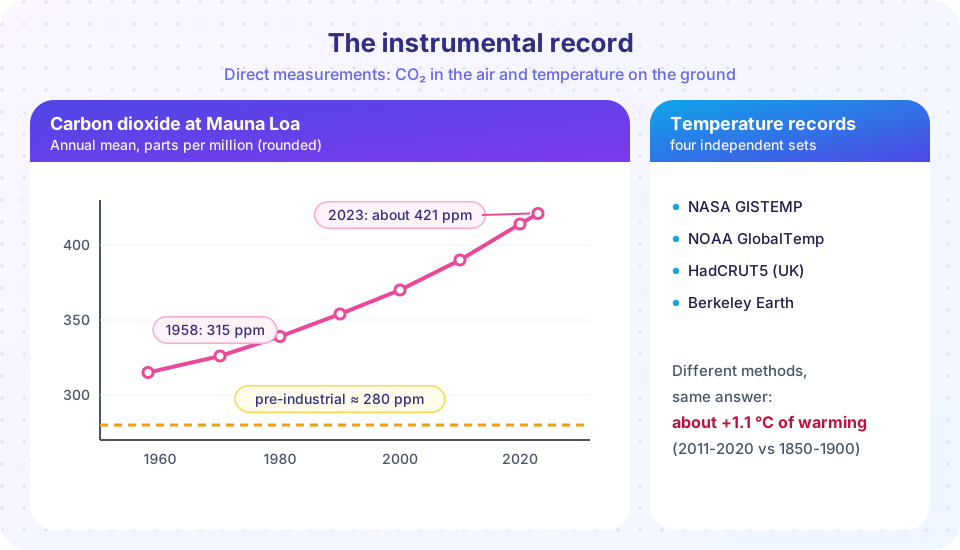
Four main groups produce global surface temperature series from largely overlapping raw data but with different methods: NASA (GISTEMP), the US National Oceanic and Atmospheric Administration (NOAA), the UK Met Office with the University of East Anglia (HadCRUT5) and Berkeley Earth. Reanalyses (like ERA5) provide a fifth, model-based approach that does not directly use the same adjustments. They disagree on year-to-year values by only a few hundredths of a degree and agree on the long-term trend. The IPCC's assessment is that global surface temperature in 2011-2020 was about 1.09 °C (likely range 0.95 to 1.20 °C) above 1850-1900. The years 2023 and 2024 were the warmest on record, with 2024 about 1.5 °C above the 1850-1900 baseline in the consolidated estimate of the World Meteorological Organization, although a single year above 1.5 °C is not the same as exceeding the long-term target in the Paris Agreement, which concerns multi-decade averages.
These surface records are not the only evidence. The upper ocean has warmed, glaciers worldwide have been shrinking, Arctic sea ice has declined, sea level has risen by about 20 cm since 1900, and spring comes earlier. Each is measured differently, and all tell the same story.
The Keeling curve
In 1958 Charles David Keeling began measuring CO₂ at the Mauna Loa Observatory in Hawaii, at 3,400 m, far from cities and forests. His instrument measured infrared absorption by CO₂ in air samples with unprecedented precision. The record shows a rise from about 315 ppm in 1958 to about 421 ppm in 2023 and over 424 ppm in 2024, with a yearly sawtooth about 6 ppm from peak (May) to trough (October), caused by Northern Hemisphere plants. The rate of rise has increased from about 0.9 ppm per year in the 1960s to over 2.4 ppm per year in the 2010s. Other stations in places such as the South Pole, Alaska and Samoa show the same trend and the same seasonal pattern, with the seasonal swing weaker in the south where there is less land.
Common misconceptions
"The temperature data are adjusted to create warming." Adjustments correct for known problems and are published with their methods. Overall they reduce the long-term global warming trend. Raw data, and data from only the best-sited stations, show the same warming.
"Satellites disagree with thermometers." Early disagreements arose from errors in the satellite analysis (orbit decay, instrument drift). With corrections, satellite lower-atmosphere and surface records agree on warming, though they measure different layers.
"Most stations are in cities, so the record is an urban artifact." The ocean record, rural stations, and sensors such as borehole temperatures and glaciers all show warming; urban areas are a small fraction of the planet.
Try it
The first example demonstrates homogenization. A synthetic station suffers a 0.6 °C downward step when it is moved in 1980. Comparing it with the average of its neighbors reveals the step; the adjusted series recovers the true trend.
Press Run (or Ctrl + Enter) to see the result here.
Program input · what you'd type while the program runs
Type the answers before you press Run, one per line. Each time the program reads a line (with input()), it gets the next line from this box.
The second example builds a global mean from a gridded field and shows why area weighting matters. The warming pattern is invented, with a stronger warming near the poles.
Press Run (or Ctrl + Enter) to see the result here.
Program input · what you'd type while the program runs
Type the answers before you press Run, one per line. Each time the program reads a line (with input()), it gets the next line from this box.
The third example estimates the effect of urban heating on the global mean from the area it covers.
Check your understanding
Quick check · 6 questions
of 6 answered You scored / 6 · perfect!
-
1. Why is a global temperature average calculated from gridded anomalies with area weighting?
The area of a latitude-longitude box shrinks with the cosine of latitude, so an unweighted mean would overweight the poles. -
2. What is homogenization?
Homogenization removes artificial steps found by comparing a station with its neighbors. -
3. How did the adjustments for sea surface temperature affect the global warming trend?
Correcting the shift from bucket to engine-intake measurements lowered the early-20th-century trend slightly overall. -
4. Which argument shows the urban heat island cannot explain global warming?
Warming appears over the oceans and in rural areas, where no urban effect exists. -
5. Roughly how large is the Keeling curve's seasonal swing in CO₂?
Northern Hemisphere plants cause a yearly sawtooth of about 6 ppm at Mauna Loa. -
6. What does the Argo network measure?
Argo floats profile the upper 2,000 m of the ocean.
Summary
- The instrumental record combines stations, ships, buoys, Argo floats and satellites; each source needs corrections and cross-checks.
- Global means are built from gridded anomalies weighted by area; homogenization removes non-climate steps.
- The urban heat island is real but local, and its effect on global trends is negligible.
- NASA, NOAA, HadCRUT5, Berkeley Earth and reanalyses agree: about +1.1 °C in 2011-2020 relative to 1850-1900.
- The Keeling curve shows CO₂ rising from about 315 ppm (1958) to over 420 ppm, with a seasonal cycle of about 6 ppm.
Next: Ice cores
Track your progress
Create a free account to tick off lessons and pick up where you left off on any device.
of Climate Science lessons completed