


















Lesson 26 of 48 · Climate Models
General circulation models and Earth system models
See how a general circulation model slices the planet into grid cells and time steps, what must be parameterized, and how models are tested against observations.
A one-number model tells you the planet's average temperature, but it cannot tell you where it will rain, how the jet stream will move, or how fast the Arctic will lose its ice. For those questions you need a general circulation model (GCM): a program that follows the winds, ocean currents, heat and moisture everywhere on the globe, moment by moment.
This lesson explains how such a model is built from the equations of fluid motion, why it needs a grid, what gets approximated rather than calculated, and how scientists test whether the result deserves trust.
What you will learn
- Name the physical laws that a GCM solves.
- Explain grid cells, vertical layers and time steps, and why resolution is expensive.
- Distinguish resolved processes from parameterized ones, with examples.
- Describe how Earth system models extend GCMs and how models are evaluated.
Key terms
GCM: a three-dimensional numerical model of the atmosphere and/or ocean. Earth system model (ESM): a GCM coupled to carbon cycle, vegetation, ice and chemistry components. Parameterization: a simple formula that represents the average effect of processes too small or too complex to resolve. Time step: how far forward in time the model moves in each calculation. Spin-up: a long preliminary run that lets the model reach a steady climate before experiments begin.
The laws behind the code
An atmosphere model solves a set of conservation laws, often called the primitive equations:
- Momentum: air accelerates because of pressure differences, gravity, the Coriolis effect of Earth's rotation, and friction (Newton's second law for a fluid).
- Mass: air is neither created nor destroyed; if it converges in one place it must rise or spread elsewhere.
- Energy: heat is moved around and changed by radiation, condensation and mixing (the first law of thermodynamics).
- Moisture: water vapor is carried by the wind and converts to cloud and rain.
- Equation of state: the ideal gas law ties pressure, density and temperature together.
The ocean uses the same laws with seawater's own equation of state, which depends on salinity as well as temperature. Sea ice, land surface and rivers have their own simpler rules. Together they form a coupled model: the atmosphere pushes the ocean with wind and heat, and the ocean feeds back through its surface temperature.
Why a grid?
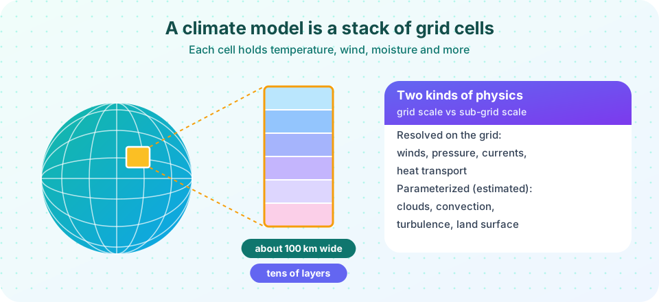
These equations cannot be solved with pen and paper for a real planet, so models solve them numerically. Cut the globe into a mesh of boxes. In each box store a handful of numbers: temperature, pressure, wind components, humidity. The equations tell you how each number changes in a short interval depending on its neighbors. Step forward, repeat millions of times, and you have a simulated climate.
A typical climate model grid in recent assessments has horizontal spacing of 50 to 250 km, with tens of vertical layers in the atmosphere (a few dozen up to about a hundred) and an ocean grid of about 0.25° to 1° (roughly 25 to 100 km). Each step might cover 10 to 30 minutes of model time. A century of simulation takes millions of steps, and each step updates every number in every box.
The cost of resolution
Halving the horizontal spacing multiplies the number of columns by four. In addition, numerical stability needs a shorter time step. An explicit scheme must obey the CFL condition (Courant, Friedrichs and Lewy, 1928): information must not travel more than one grid cell in one step. Halve the cell and you must halve the step. So the work grows by about 4 × 2 = 8. Doubling the vertical layers adds another factor of two. That is why climate-length simulations use grids far coarser than modern weather forecasts, and why running the next generation of models often needs a new supercomputer.
What is resolved and what is parameterized
A 100 km grid box can resolve a hurricane's larger structure only crudely and a thunderstorm not at all. Many important processes happen at smaller scales than the grid. The model does not ignore them; it uses a parameterization, a compact rule that estimates the net effect of the small-scale process on the grid-scale numbers.
| Process | Why it is sub-grid | Typical approach |
|---|---|---|
| Convection and thunderstorms | Updrafts are a few kilometers wide | Rules for when and how much heat and moisture rises |
| Clouds | Droplets form on microscopic scales | Cloud fraction and optical depth from humidity and temperature |
| Turbulence near the surface | Eddies are meters to hundreds of meters | Mixing coefficients |
| Ocean eddies (in coarse models) | About 10 to 100 km | Parameterized stirring of heat and salt |
| Land surface | Vegetation, soil moisture vary locally | Land-surface sub-models |
| Aerosols | Particles are microscopic | Prescribed or computed concentrations that scatter or absorb sunlight |
Parameterizations contain numbers that cannot be derived exactly from first principles and are chosen using observations. This is called tuning. Responsible modeling centers document their tuning choices, and a few have published the targets they tune to (for example, the top-of-atmosphere energy balance). Cloud parameterization remains the largest source of difference between models in their warming response.
Higher resolution to the rescue?
Some research models now run at 1 to 10 km resolution so that convection is resolved directly, at least in part of the globe. These "storm-resolving" models are expensive and cannot yet run for centuries, but they are changing how scientists test and improve parameterizations.
From GCM to Earth system model
A plain atmosphere-ocean GCM is told how much CO₂ is in the air. An Earth system model calculates it. It adds:
- an ocean carbon cycle (CO₂ dissolving, plankton, sinking carbon);
- a land carbon cycle (photosynthesis, soil respiration, fire, vegetation shifts);
- dynamic ice sheets in some models;
- atmospheric chemistry (ozone, methane lifetime) and aerosols.
This lets the model study feedbacks between climate and the carbon cycle: if warmer soils release more CO₂, the model sees it. About half of human CO₂ emissions have stayed in the air and the rest has been taken up by oceans and land. An ESM can ask whether that will continue.
Running the model: spin-up, drift and ensembles
A new model starts from rough initial conditions. It is run for hundreds or thousands of simulated years under constant preindustrial conditions, the spin-up, until the deep ocean stops adjusting and the climate stops drifting. This control run also shows the model's own internal variability, such as El Niño-like swings. Experiments then branch off from it: historical forcing from 1850 onward, then future scenarios.
Because the climate system is chaotic, scientists run the same experiment several times with tiny differences in the start. This initial-condition ensemble separates the forced signal from random weather. Coordinating many centers is the job of the Coupled Model Intercomparison Project (CMIP), whose sixth phase (CMIP6) provided the simulations used in the IPCC's Sixth Assessment Report.
How do we know the model is any good?
Scientists evaluate models in several ways.
- Climatology: does the model produce the observed seasons, jet streams, monsoons, deserts and ocean currents?
- Variability: does it generate El Niño, the North Atlantic Oscillation and realistic extremes?
- Hindcasts: given the real forcing from 1850 to today (volcanoes, solar changes, greenhouse gases, aerosols), does it reproduce the observed global temperature curve? Multi-model averages do this well, including the cooling after large volcanic eruptions such as Mount Pinatubo in 1991.
- Past climates: can it simulate the last ice age or the warm mid-Pliocene?
- Prediction tests: the 1988 projections of James Hansen and the 1990 IPCC report have been compared with later observations, and several analyses found that the models' projected warming was close to what happened once the actual emissions were used.
- Process tests: field campaigns measure clouds, convection and ocean mixing directly.
Known weaknesses
No model is perfect. Many have a double ITCZ bias, with too much rain south of the equator in the Pacific. Some produce too little Arctic amplification or too weak Atlantic circulation variability. Models struggle with small-scale extreme rainfall and tropical cyclone intensity. A smaller set of "hot models" in CMIP6 had climate sensitivities higher than the range supported by other lines of evidence, and the IPCC down-weighted them in its assessed warming ranges.
Common misconceptions
"Models are tuned to match the warming trend." Models are tuned on climate-mean quantities such as the energy balance, not on the 20th-century warming curve. Matching the warming is a test result, not a fitting target.
"Parameterization means guessing." A parameterization is an approximation grounded in observations and theory, tested against data. It does add uncertainty, which scientists estimate by comparing models.
"Better resolution always means better answers." Higher resolution helps with some features (storms, mountains, coastlines) and does not cure all errors. Physics matters as much as grid size.
Try it
The first demonstration shows the CFL limit. A heat-diffusion calculation is stable when the time step is small enough and blows up when it is too big, just as a climate model would.
Press Run (or Ctrl + Enter) to see the result here.
Program input · what you'd type while the program runs
Type the answers before you press Run, one per line. Each time the program reads a line (with input()), it gets the next line from this box.
The second demonstration shows why resolution matters for a moving feature. The same pulse is carried by a wind across a coarse and a fine grid. The coarse grid smears it out.
Press Run (or Ctrl + Enter) to see the result here.
Program input · what you'd type while the program runs
Type the answers before you press Run, one per line. Each time the program reads a line (with input()), it gets the next line from this box.
Check your understanding
Quick check · 5 questions
of 5 answered You scored / 5 · perfect!
-
1. What does a parameterization do?
Parameterizations estimate the net effect of processes, such as convection, that are smaller than a grid cell. -
2. Halving horizontal grid spacing in a model needs roughly how much more computing?
Four times as many columns, and the shorter time step needed for stability roughly doubles the number of steps. -
3. What is the extra ingredient of an Earth system model compared with a plain GCM?
ESMs compute CO₂ and related cycles instead of being told the concentration. -
4. Why is a spin-up run needed?
The deep ocean takes centuries to adjust. Spin-up removes drift so experiments reveal real responses. -
5. Which is a test of a model that does NOT involve fitting to the 20th-century warming curve?
Climatology, variability and process tests judge the physics independently of the warming trend.
Summary
- GCMs solve the conservation laws for momentum, mass, energy and moisture on a 3-D grid.
- Resolution is costly: halving the spacing costs about eight times more.
- Sub-grid processes such as clouds and convection are parameterized and are a main source of uncertainty.
- Earth system models add carbon, vegetation, ice and chemistry.
- Models are evaluated through climatology, variability, hindcasts, past climates and process studies.
Track your progress
Create a free account to tick off lessons and pick up where you left off on any device.
of Climate Science lessons completed