


















Lesson 48 of 48 · Projects and Practice
Further Study: Where to Go After Circuit Analysis
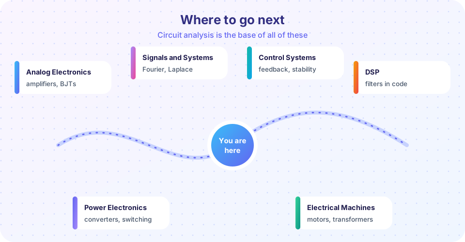
A roadmap from circuit analysis to analog electronics, signals and systems, control, power electronics, DSP and machines, with a pole preview and a path chooser.
You can now analyze resistive networks, predict how circuits settle after a switch, handle sinusoidal steady state with phasors and design simple filters and resonators. That is the foundation of all electrical and electronic engineering. This last lesson shows how the ideas you learned reappear in later subjects, so you can choose your next step with a clear picture of what each one adds.
What you will learn
- Which subjects build directly on circuit analysis and why.
- A preview of the idea that connects them: poles and the complex frequency
s. - A realistic study plan and project ideas.
Key terms
Complex frequency s: σ + jω; the Laplace-transform variable that treats decay and oscillation together.
Pole: a value of s where a transfer function becomes infinite; it sets the natural behavior of the circuit.
Active circuit: one containing amplifying devices (transistors, op-amps), as opposed to passive R, L, C.
System: a general input-output relationship, of which a circuit is one example.
Six directions
Analog electronics. Add transistors and op-amps and circuits gain the ability to amplify. Your tools carry over directly: small-signal analysis replaces each transistor by a linear model (resistors and dependent sources), then you apply nodal analysis, Thévenin equivalents and Bode plots. See the Analog Electronics track.
Signals and systems. The sinusoids of chapter 7 are a special case. Fourier series and transforms say that any signal is a sum of sinusoids, so the frequency response H(jω) from chapter 8 describes how a system treats any signal. The Laplace transform extends it to transients. See Signals and Systems.
Control systems. Feedback uses the transfer function in a loop. The Bode plot, phase margin and the damping ratio from the RLC lesson become the main tools for deciding whether a system is stable and how fast it responds. See Control Systems.
Digital signal processing. Filters you built from R, L and C can be reproduced in software by working on samples. The RC low-pass becomes a one-line recursive formula. See Digital Signal Processing.
Power electronics and machines. Switching converters use inductors and capacitors with fast switches to change voltages efficiently, and three-phase power uses the complex power of chapter 7. See Power Electronics and Electrical Machines.
Building real things. To turn calculations into hardware, try Arduino for microcontroller projects and PCB Design for putting circuits on a board.
Supporting mathematics helps in every direction: Differential Equations explains where e^(−t/τ) comes from, Linear Algebra underlies nodal analysis of big networks, and Complex Analysis deepens the idea of poles.
The idea that connects them: poles
In chapter 6 the series RLC circuit had two roots s = −α ± √(α² − ω₀²). Those are the poles of its transfer function 1/(LC s² + RC s + 1). Each pole s = σ + jω contributes a response e^(σt) that oscillates at ω and decays (if σ < 0) at rate |σ|. Real poles give exponentials, complex pairs give ringing, and poles in the right half-plane mean instability. Every subject on the map above uses this picture. Resonance, damping, cutoff frequency and settling time are all properties of pole locations.
A study plan
- Weeks 1–2. Redo the practice problems without notes; build the solver from the project lesson from memory.
- Weeks 3–6. Learn the Laplace transform and poles in Signals and Systems; reproduce the RLC results with it.
- Weeks 7–12. Pick one direction: electronics if you like building, control if you like feedback, DSP if you like programming.
- Always. Build something: a filter on a breadboard, a power-factor measurement, a simple radio tuner. Measured results teach what equations do not.
Common misconceptions
"Circuit analysis is finished once I pass the exam." It is the language of the next ten subjects; time spent making it automatic is never wasted.
"Simulators make hand analysis obsolete." Simulators give numbers. Hand analysis gives understanding and tells you whether the simulator's answer is plausible.
"Only electrical engineers need this." Mechanical systems (springs and dampers), thermal systems and even some biology models follow the same mathematics.
Try it
The first program previews the pole picture. For the series RLC circuit it finds the poles of the transfer function with numpy.roots for three resistances and classifies the response, exactly as you did by hand in chapter 6.
Press Run (or Ctrl + Enter) to see the result here.
Program input · what you'd type while the program runs
Type the answers before you press Run, one per line. Each time the program reads a line (with input()), it gets the next line from this box.
The second tool is a small path chooser: pick your main interest and it suggests which track on this site to study next.
Check your understanding
Quick check · 4 questions
of 4 answered You scored / 4 · perfect!
-
1. Which subject uses the transfer function H(jω) to describe how a system treats any signal, by splitting it into sinusoids?
Fourier analysis writes a signal as a sum of sinusoids, and H(jω) acts on each one. -
2. A complex pair of poles in the left half-plane means the response
The imaginary part gives oscillation and the negative real part gives decay: ringing. -
3. In small-signal analysis of an amplifier, transistors are replaced by
Linear models let you apply nodal analysis, Thévenin equivalents and Bode plots. -
4. Why is understanding poles useful across subjects?
Pole locations determine the natural responses of any linear system.
Summary
- Analog electronics, signals and systems, control, DSP, power electronics and machines all build on circuit analysis.
- Poles in the complex plane unify resonance, damping and stability.
- Practice by building things and by re-deriving results in a new language (Laplace).
- Keep your hand-analysis skills: they tell you when a simulator is lying.
Next: back to the Circuit Analysis course page
Track your progress
Create a free account to tick off lessons and pick up where you left off on any device.
of Circuit Analysis lessons completed