


















Lesson 13 of 47 · Transmission Lines
Short and Medium Lines: Series Model, Nominal Pi and ABCD
Model short and medium transmission lines with the series impedance and nominal pi circuits, use ABCD constants, and compute voltage regulation, losses and efficiency.
With the per-kilometer constants from the previous lesson, you can build a circuit model of an entire line. The right model depends on length. For short lines the capacitance is negligible and a single series impedance is enough. For medium lines the capacitance matters, so we add shunt branches. Either way, the model lets you answer the practical questions: what sending-end voltage do I need to hold the receiving end at rated value, how much power is lost, and how does the voltage change with load?
What you will learn
- How to use the short-line model and compute voltage regulation.
- How to build the nominal-π model and find its ABCD constants.
- How to find sending-end voltage, current, power, losses and efficiency.
- How power factor changes the voltage drop along a line.
Key terms
- Series impedance Z:
(r + jx) × length, the total resistance and reactance of the line. - Shunt admittance Y:
j b × length, the total charging susceptance. - ABCD constants: the four complex numbers relating sending and receiving quantities:
Vs = A Vr + B Ir,Is = C Vr + D Ir. - Voltage regulation:
(|Vr,NL| − |Vr,FL|) / |Vr,FL|, the voltage rise from full load to no load. - Sending end / receiving end: the generator side and the load side of the line.
The short line (up to about 80 km)
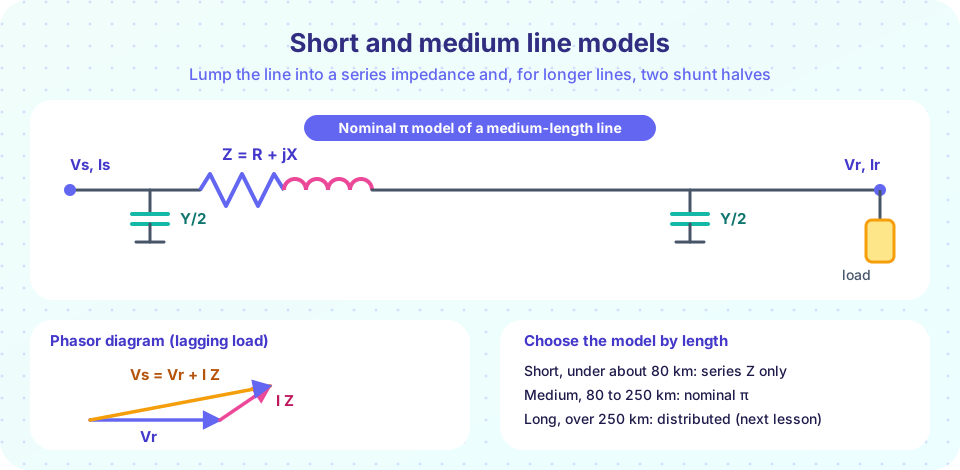
At low voltage and short length, the shunt capacitance carries a negligible current, so the line is just the total series impedance Z = R + jX. Currents at both ends are equal, and
Vs = Vr + Z × Ir, Is = Ir
All quantities are per phase (line-to-neutral voltages). The ABCD constants are A = D = 1, B = Z, C = 0.
Worked example. A 60 km, 132 kV line has z = 0.1 + j0.4 Ω/km, so Z = 6 + j24 Ω. It delivers 100 MW at power factor 0.9 lagging with Vr = 132 kV line-to-line.
Vr = 132000 / √3 = 76,210 Vper phase (reference at 0°).Ir = 100×10⁶ / (√3 × 132,000 × 0.9) = 486 Aat−25.8°.Vs = Vr + Z Ir = 84,424 Vper phase at6.3°, which is146.2 kVline-to-line.- Voltage regulation with the load removed (receiving end rises to
Vs):(84,424 − 76,210) / 76,210 = 10.8%. - Line loss
3 |Ir|² R = 3 × 486² × 6 = 4.25 MW, so the efficiency is100 / (100 + 4.25) = 95.9%.
The power factor changes the answer. At unity power factor the regulation is 4.4%. With the same 100 MW at 0.9 leading, it is about −2%: the receiving voltage actually rises above the sending voltage. A leading load acts like a capacitor, which pushes the voltage up along an inductive line.
The medium line (about 80 to 250 km)
At longer lengths, the line's charging current can no longer be ignored. The nominal-π model puts the whole series impedance Z in the middle and splits the shunt admittance Y = j b × length into two halves, Y/2 at each end. (A nominal-T model does the opposite, with Z/2 on each side and Y in the middle; the two are close but not identical.)
Applying Kirchhoff's laws to the π circuit gives the ABCD constants:
A = D = 1 + Z Y / 2B = ZC = Y (1 + Z Y / 4)
and a reciprocal two-port always satisfies A D − B C = 1, which is a handy check. Sending-end values follow from
Vs = A Vr + B Ir, Is = C Vr + D Ir
At no load, Ir = 0, so Vr,NL = Vs / A, and the voltage regulation is VR = (|Vs| / |A| − |Vr,FL|) / |Vr,FL|.
Worked example. A 150 km, 220 kV line has z = 0.08 + j0.40 Ω/km and y = j2.8 µS/km. So Z = 12 + j60 Ω and Y = j420 µS. It delivers 150 MW at power factor 0.85 lagging at 220 kV.
A = D = 1 + ZY/2 = 0.9874 + j0.0025,B = Z,C = −0.5×10⁻⁶ + j417×10⁻⁶ S.Ir = 150×10⁶ / (√3 × 220,000 × 0.85) = 463 Aat−31.8°.Vs = A Vr + B Irgives253.4 kVline-to-line at an angle of8.3°, andIs = 432 A.- No-load receiving voltage
Vs / |A| = 148.2 kVper phase versus 127 kV full load: regulation16.7%. - Sending-end power
157.3 MW, so the loss is7.3 MWand the efficiency95.4%.
The regulation is large because 150 MW is close to this line's natural loading (lesson 4 of this chapter). Real operators use shunt capacitors, tap changers and generator excitation to hold voltage.
Choosing a model
The length limits are guides, not laws. Use the short model when the charging current is a negligible fraction of the load current. Use the π model when the line's charging reactive power matters, which happens at higher voltage because charging current grows with V. For lines longer than about 250 km, or whenever you need accuracy, use the distributed model from the next lesson.
Common misconceptions
- "Voltage always drops along a line." With a leading load, or on a lightly loaded line where charging current dominates, the receiving-end voltage can exceed the sending-end voltage.
- "Efficiency of a line equals its voltage regulation." They are different measures. Regulation is about voltage; efficiency compares power out with power in.
- "The two halves Y/2 in the π model are the same as two capacitors on each wire." They represent the total shunt effect of the line, lumped at the ends.
Try it
First, vary the power factor on the short-line example and plot the voltage regulation. This shows how strongly the load's reactive power influences voltage.
Press Run (or Ctrl + Enter) to see the result here.
Program input · what you'd type while the program runs
Type the answers before you press Run, one per line. Each time the program reads a line (with input()), it gets the next line from this box.
Second, solve the medium line with ABCD constants and sweep the delivered power. The plot shows how the sending-end voltage required to hold 220 kV at the load climbs with loading. The code also checks A D − B C = 1.
Press Run (or Ctrl + Enter) to see the result here.
Program input · what you'd type while the program runs
Type the answers before you press Run, one per line. Each time the program reads a line (with input()), it gets the next line from this box.
Check your understanding
Quick check · 5 questions
of 5 answered You scored / 5 · perfect!
-
1. In the short-line model, what are the ABCD constants?
With no shunt branch, Vs = Vr + Z Ir and Is = Ir, so A = D = 1, B = Z and C = 0. -
2. A short line has Z = 4 + j12 Ω. At Ir = 100 A at 0° (unity pf) and Vr = 11 kV per phase, what is |Vs| approximately?
Z Ir = 400 + j1200 V, so Vs = 11,400 + j1200 V and |Vs| = √(11,400² + 1200²) = 11,463 V. Adding the magnitudes of the drop directly (11.0 + 1.27 = 12.27 kV) would overestimate it. -
3. Which of the following is always true for a medium line modeled as a nominal π?
For any passive reciprocal two-port, A D − B C = 1. -
4. Why can the receiving-end voltage exceed the sending-end voltage?
Capacitive (leading) current through an inductive line raises the voltage. This is the Ferranti effect. -
5. Which line length range usually calls for a nominal-π model?
That is the usual range where charging current matters but a lumped model is still accurate enough.
Summary
- Short line:
Vs = Vr + Z Ir,A = D = 1,B = Z,C = 0. - Nominal π:
A = D = 1 + ZY/2,B = Z,C = Y(1 + ZY/4), andAD − BC = 1. - Voltage regulation depends strongly on the load power factor; leading loads can make it negative.
- Line loss is
3 I² R; efficiency is power out over power in. - Pick the model by length; use the distributed model beyond about 250 km.
Track your progress
Create a free account to tick off lessons and pick up where you left off on any device.
of Electric Power Systems lessons completed