


















Lesson 14 of 47 · Transmission Lines
Long Lines and Surge Impedance Loading
Model long transmission lines with distributed parameters, understand the propagation constant, characteristic impedance, the Ferranti effect and surge impedance loading.
For lines longer than about 250 km, lumping the parameters into one impedance and one pair of shunt branches stops being accurate. The resistance, inductance and capacitance are spread continuously along the line, and a voltage change at one end travels along it as a wave. The correct model uses hyperbolic functions. It looks more complicated, but it gives you three ideas that matter in every real grid: the characteristic impedance, the Ferranti voltage rise, and the surge impedance loading, the load at which a line neither makes nor uses reactive power.
What you will learn
- How to write the long-line equations with
γandZc. - What the propagation constant, wavelength and velocity mean.
- Why a lightly loaded long line has a voltage rise (the Ferranti effect).
- What surge impedance loading is and how it relates to stability limits.
Key terms
- Propagation constant (γ):
γ = √(z y) = α + jβ;αis attenuation,βis the phase shift per kilometer. - Characteristic (surge) impedance (Zc):
Zc = √(z / y); the ratio of voltage to current for a wave traveling on the line. - Surge impedance loading (SIL):
SIL = VLL² / Zc, the power delivered into a load equal toZc. - Ferranti effect: the voltage rise at the open end of a long, lightly loaded line.
- Wavelength: the distance over which the phase shift reaches 2π, about 6000 km at 50 Hz and 5000 km at 60 Hz.
The distributed model
With series impedance per kilometer z = r + jωL and shunt admittance per kilometer y = g + jωC (g is nearly zero), the voltage and current at distance x from the receiving end satisfy two coupled differential equations. Their solution at the sending end of a line of length l is
Vs = Vr cosh(γ l) + Zc Ir sinh(γ l)
Is = (Vr / Zc) sinh(γ l) + Ir cosh(γ l)
so the exact ABCD constants are A = D = cosh(γ l), B = Zc sinh(γ l) and C = sinh(γ l) / Zc.
For the 400 kV line of lesson 2 (L = 1.022 mH/km, C = 11.16 nF/km, with r = 0.03 Ω/km added), the numbers are Zc ≈ 303 Ω (with a small negative imaginary part from the resistance) and γ ≈ 5×10⁻⁵ + j1.062×10⁻³ per km. The attenuation is tiny: most of γ is the phase constant β.
Lossless line: waves in plain sight
Ignoring r and g makes γ = jβ with β = ω √(L C), and Zc = √(L / C) becomes a real resistance. For the example, β = 1.061×10⁻³ rad/km = 0.0608°/km. The wave travels at v = 1 / √(LC) ≈ 2.96×10⁵ km/s, nearly the speed of light, and the wavelength is 2π / β ≈ 5922 km. A 300 km line is therefore about one twentieth of a wavelength long, or βl = 18.2° electrically.
The hyperbolic functions become trigonometric: cosh(jβl) = cos βl and sinh(jβl) = j sin βl.
Accuracy of the simpler models
The nominal-π model can be corrected to match the exact solution at the terminals by scaling Z and Y:
Z' = Z × sinh(γ l) / (γ l), Y'/2 = (Y / 2) × tanh(γ l / 2) / (γ l / 2)
For the example line carrying 600 MW at power factor 0.95 lagging at 400 kV, delivered over 300 km, the exact sending-end voltage is 461.3 kV, at an angle of 17.6°. The uncorrected nominal π gives 463.0 kV, an error of 0.4%. The corrected π matches the exact value. For shorter lines the error is smaller; beyond about 400 km it grows quickly.
The Ferranti effect
Open the receiving end: Ir = 0. Then Vs = Vr cos(βl) for a lossless line, so
Vr = Vs / cos(βl)
The receiving-end voltage is higher than the sending-end voltage. For l = 300 km, βl = 18.2°, cos βl = 0.950, so Vr = 1.053 Vs: a 5.3% rise on an open line. For 600 km it would be 1 / cos 36.5° = 1.24, which is dangerous. The rise comes from the charging current flowing through the line's inductance. Operators control it with shunt reactors, which absorb the charging reactive power, and by never energizing a long line at the end of a weak network without care.
Surge impedance loading
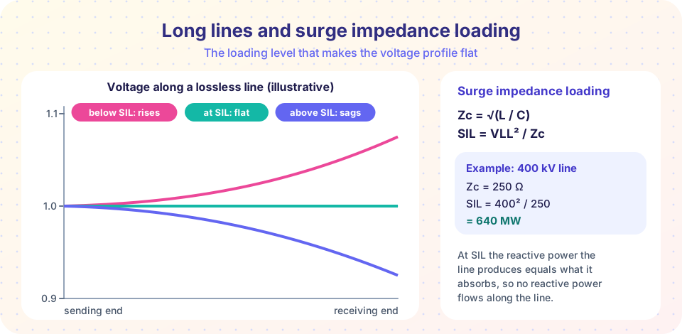
If the line feeds a load of resistance Zc, then Vr = Zc Ir, and for a lossless line the voltage and current along the line keep the same magnitude everywhere, shifting only in phase. The reactive power absorbed by the series inductance equals the reactive power produced by the shunt capacitance, so no reactive power flows along the line. The power delivered is
SIL = VLL² / Zc
For the example line, SIL = 400² / 302.6 = 529 MW. Typical values are 130 to 150 MW for a 230 kV line, 400 to 500 MW at 345 kV and 2000 MW or more at 765 kV.
- Loaded below SIL: the line produces more reactive power (capacitive) than it absorbs, and the voltage tends to rise in the middle and toward the receiving end.
- Loaded above SIL: the line absorbs reactive power, and the voltage sags unless supported.
SIL is a handy benchmark: short lines can carry several times SIL (limited by heat), medium lines up to about two to three times, and very long lines only about SIL or less. The theoretical steady-state limit of a lossless line is
Pmax = Vs Vr / (Zc sin βl)
For the 300 km example this equals 1689 MW, about 3.2 SIL. For 600 km it falls to 889 MW, about 1.7 SIL. Practical limits are lower because stable operation requires margin against disturbances; chapter 6 explains why.
Common misconceptions
- "SIL is the maximum a line can carry." It is a benchmark for voltage behavior, not a limit. Short lines carry multiples of it, and very long lines must stay near or below it.
- "A line loaded at SIL has no current." It has the full current; what vanishes is the net reactive power flow along the line.
- "The Ferranti effect only occurs in cables." It occurs on any lightly loaded long line, and is stronger on cables because their capacitance is higher.
Try it
First, compare the exact long-line model with the short-line, nominal-π and corrected-π models as the length of the example line grows. The plot shows the error of each in the sending-end voltage.
Press Run (or Ctrl + Enter) to see the result here.
Program input · what you'd type while the program runs
Type the answers before you press Run, one per line. Each time the program reads a line (with input()), it gets the next line from this box.
Second, plot the voltage profile along the lossless line for several loadings, and print the Ferranti rise. The profile uses |V(x)| / Vr = √(cos²(βx) + k² sin²(βx)) for a unity-power-factor load, where k = P / SIL and x is the distance from the receiving end.
Press Run (or Ctrl + Enter) to see the result here.
Program input · what you'd type while the program runs
Type the answers before you press Run, one per line. Each time the program reads a line (with input()), it gets the next line from this box.
Third, a quick explorer for how line length changes the Ferranti rise and the theoretical power limit as a multiple of SIL, using the lossless formulas.
Check your understanding
Quick check · 5 questions
of 5 answered You scored / 5 · perfect!
-
1. A lossless line has L = 1.2 mH/km and C = 10 nF/km. What is its characteristic impedance?
Zc = √(L / C) = √(1.2×10⁻³ / 10×10⁻⁹) = √(120,000) = 346 Ω. -
2. What is the SIL of a 345 kV line with Zc = 300 Ω?
SIL = 345² / 300 = 119,025 / 300 = 397 MW. -
3. A lossless line is open at the receiving end and βl = 20°. By what factor is Vr larger than Vs?
Vr / Vs = 1 / cos 20° = 1.064. -
4. A line carries more than its SIL. What happens to the reactive power?
Above SIL, the series inductance absorbs more reactive power than the shunt capacitance produces. -
5. Shunt reactors are installed on long lines mainly to:
The reactors absorb the reactive power generated by the line capacitance when the line is lightly loaded.
Summary
- Long lines use distributed parameters:
Vs = Vr cosh γl + Zc Ir sinh γl. Zc = √(z / y)andγ = √(z y) = α + jβ; the wavelength is about 6000 km at 50 Hz.- A corrected π reproduces the exact solution; the uncorrected π is accurate to a fraction of a percent at 300 km.
- Ferranti effect:
Vr = Vs / cos βlon an open lossless line. SIL = VLL² / Zc; at SIL the voltage profile is flat and no reactive power flows along the line.
Next: Chapter 3 Review
Track your progress
Create a free account to tick off lessons and pick up where you left off on any device.
of Electric Power Systems lessons completed