


















Lesson 19 of 47 · Per-Unit Analysis and Load Flow
Newton-Raphson Load Flow: Bus Types, Jacobian and DC Approximation
Learn load flow: slack, PV and PQ buses, the power-flow equations, the Newton-Raphson iteration with the Jacobian, a 3-bus example solved in Python, and the DC approximation.
A load flow answers the central operating question: given the generation and the demand, what are the voltage and the angle at every bus, and how much power flows on every line? With Ybus in hand the equations are easy to write but impossible to solve with algebra alone, because the unknown voltages appear in products and cosines. The industry standard is the Newton-Raphson method, which turns a nonlinear problem into a short sequence of linear ones.
What you will learn
- The three bus types and which quantities are known at each.
- How power mismatches define the equations to be solved.
- How a Newton-Raphson iteration with the Jacobian works.
- How the DC load flow simplifies the problem, and when it is accurate.
Key terms
- Slack bus: the reference bus where
|V|andδare fixed; it absorbs the losses. - PV bus: a generator bus where
Pand|V|are specified. - PQ bus: a load bus where
PandQare specified. - Mismatch: the difference between the specified and the calculated power at a bus.
- Jacobian (J): the matrix of partial derivatives of the mismatches with respect to the unknowns.
Bus types and unknowns
Each bus has four variables: P, Q, |V| and δ. Two are specified, two are unknown.
| Bus type | Specified | Unknown | Typical use |
|---|---|---|---|
| Slack | voltage magnitude and angle | P, Q |
one reference generator |
| PV | P and voltage magnitude |
Q, angle |
generators with voltage control |
| PQ | P, Q |
voltage magnitude and angle | loads and fixed-output sources |
Why a slack bus? The total generation must equal the total load plus the losses, but the losses depend on the solution, so someone must be left free to supply the difference. The slack bus does, and its angle sets the reference for all others.
For n buses with one slack, n − 1 real-power equations and one reactive-power equation for each PQ bus are needed. From the previous lesson,
Pi = Σj |Vi||Vj| (Gij cos θij + Bij sin θij)
Qi = Σj |Vi||Vj| (Gij sin θij − Bij cos θij)
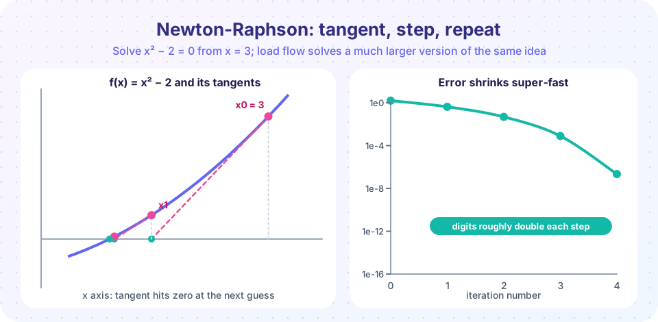
Newton-Raphson in one variable
To solve f(x) = 0 from a starting guess x0, replace the curve with its tangent: f(x0) + f'(x0)(x1 − x0) = 0, which gives
x1 = x0 − f(x0) / f'(x0)
and repeat. For f(x) = x² − 2 from x0 = 3, the iterates are 1.833, 1.462, 1.415 and 1.4142: each is much closer than the last. This is quadratic convergence: near the solution the number of correct digits roughly doubles each iteration.
Newton-Raphson for load flow
The unknowns form a vector x = [δ (all non-slack buses); |V| (PQ buses)]. The mismatches are
ΔPi = Pi,spec − Pi,calc for every non-slack bus
ΔQi = Qi,spec − Qi,calc for every PQ bus
The linearized update is
[ΔP; ΔQ] = J × [Δδ; Δ|V|], with J = [J1 J2; J3 J4]
where J1 = ∂P/∂δ, J2 = ∂P/∂|V|, J3 = ∂Q/∂δ and J4 = ∂Q/∂|V|. The full algorithm:
- Choose a starting guess, typically a flat start: all
|V| = 1.0(or the specified values at PV buses) and allδ = 0. - Compute
PcalcandQcalcfrom the current voltages, then the mismatches. - If the largest mismatch is below a tolerance (for example
10⁻⁶ pu), stop. - Build
Jand solve the linear system forΔδandΔ|V|. - Update the voltages and return to step 2.
Real programs build J from the sparse structure of Ybus and solve with sparse factorization, so networks of tens of thousands of buses solve in a fraction of a second. After convergence, compute the slack bus P and Q, the generator Q at PV buses, the line flows and the losses. If a PV bus needs more reactive power than its generator can supply, the program converts it to a PQ bus at its limit.
Worked example
Using the three-bus network from the previous lesson. Bus 1 is the slack with V1 = 1.04∠0°. Bus 2 is a PV generator with P2 = +0.30 pu injected and |V2| = 1.02. Bus 3 is a PQ load with P3 = −0.90 pu and Q3 = −0.30 pu (negative injection means consumption). The unknowns are δ2, δ3 and |V3|, so J is 3 × 3. A flat start gives a largest mismatch of 0.733 pu.
| Iteration | Largest mismatch (pu) | V3 (pu) | Angle at bus 2 | Angle at bus 3 |
|---|---|---|---|---|
| 0 (start) | 0.733 | 1.0000 | 0° | 0° |
| 1 | 0.0139 | 0.9977 | −0.231° | −2.423° |
| 2 | 0.0000125 | 0.9968 | −0.247° | −2.440° |
| 3 | 1.0×10⁻¹¹ | 0.9968 | −0.247° | −2.440° |
Three iterations are enough, and the mismatch falls by a few orders of magnitude each time. The results:
- Slack bus supplies
0.618 + j0.523 pu(61.8 MW and 52.3 Mvar on 100 MVA). - Bus 2 must absorb
0.168 puof reactive power (Q2 = −0.168 pu) to hold its voltage at 1.02. - Line flows: 1 to 2 carries
0.173 + j0.289, 1 to 3 carries0.446 + j0.234, 2 to 3 carries0.471 + j0.115. - Total losses:
0.0182 + j0.0547 pu. The slack bus supplies0.618 puwhile the net load is0.9 − 0.3 = 0.6 pu: the extra0.018 puis exactly the loss.
Fast-decoupled and DC load flow
In high-voltage networks, P is strongly tied to the angles and Q to the voltage magnitudes, so J2 and J3 are small. Ignoring them (with other approximations) gives the fast-decoupled load flow, which reuses two constant matrices and converges in a few cheaper iterations.
The DC load flow goes further: assume |V| = 1.0 everywhere, neglect resistance and reactive power, and use sin θ ≈ θ. Then
P = B' × δ, where B' is built from the line reactances (1/x instead of y), and the line flow is Pij = (δi − δj) / xij.
This is a single linear solve with no iteration, ideal for contingency screening and market studies. For our example the DC solution gives line flows of 0.167, 0.433 and 0.467 pu, close to the AC values of 0.173, 0.446 and 0.471 pu, but it cannot give voltages, reactive power or losses, and the angles are less accurate (−0.57° and −2.98° against −0.25° and −2.44°).
Common misconceptions
- "The slack bus is a real, special generator." It is a modeling convenience. In real operation many generators share the balancing duty (chapter 6).
- "Newton-Raphson always converges." It usually does from a flat start, but badly stressed or badly scaled networks may diverge, and a very heavily loaded network may have no solution at all.
- "DC load flow means direct current." It is the name for the linearized AC problem. There is no DC circuit involved.
Try it
First, a complete Newton-Raphson solver for the worked example. It prints the mismatch at each iteration, the final voltages, the bus powers and the line flows, and plots the mismatch on a log scale. Edit the specified powers and see how the solution moves.
Press Run (or Ctrl + Enter) to see the result here.
Program input · what you'd type while the program runs
Type the answers before you press Run, one per line. Each time the program reads a line (with input()), it gets the next line from this box.
Second, try the one-variable method yourself. Choose a function and a starting guess, and the table lists each iterate. Notice how a starting point near the root converges in a few steps and a poor start can wander.
Check your understanding
Quick check · 6 questions
of 6 answered You scored / 6 · perfect!
-
1. Which quantities are specified at a PV bus?
PV buses have a generator that fixes P and holds |V|; Q and δ are computed. -
2. Why does a load-flow study need a slack bus?
Total generation = load + losses, and losses depend on the solution. The slack bus balances them and provides the reference angle. -
3. A network has 1 slack bus, 2 PV buses and 5 PQ buses. How many unknowns does the Newton-Raphson solution have?
Angles at the 7 non-slack buses plus magnitudes at 5 PQ buses: 7 + 5 = 12. -
4. What is a 'flat start'?
A flat start initializes the unknown voltages at 1.0 pu and 0 degrees. -
5. The DC load flow assumes which of the following?
It linearizes the problem: |V| = 1, R neglected, sin θ ≈ θ. -
6. Quadratic convergence of Newton-Raphson means that near the solution:
That is why a few iterations are enough in practice.
Summary
- Each bus is slack (
|V|,δknown), PV (P,|V|known) or PQ (P,Qknown). - Newton-Raphson solves the nonlinear power equations by repeatedly solving
[ΔP; ΔQ] = J [Δδ; Δ|V|]. - It converges quadratically, typically within 3 to 6 iterations from a flat start.
- After convergence, compute slack power, generator reactive power, line flows and losses.
- Fast-decoupled and DC load flows trade accuracy for speed.
Next: Chapter 4 Review
Track your progress
Create a free account to tick off lessons and pick up where you left off on any device.
of Electric Power Systems lessons completed