


















Lesson 32 of 47 · Renewables and Storage
Solar and wind power
Learn how a solar module and a wind turbine convert energy to electricity: I-V curves, MPPT, temperature effects, the cube law, the Betz limit, Weibull statistics and capacity factor.
Solar panels and wind turbines are the two workhorses of the new grid. They turn very different energy flows into electricity, but the engineering questions are alike: how much power does the device deliver for a given sunshine or wind speed, how should it be controlled to extract the most, and how much energy will it produce in a year? Answering them lets you size a plant, estimate its revenue and predict what it will do to the grid.
This lesson builds simple but accurate models of both machines and uses them to estimate annual energy.
What you will learn
- Describe a PV module with its I-V curve, fill factor and efficiency.
- Explain why MPPT is needed and how temperature affects output.
- Use
P = ½ρA·v³·Cpand the Betz limit for wind turbines. - Estimate annual energy and capacity factor for both technologies.
Key terms
STC: standard test conditions for modules, 1,000 W/m² irradiance, 25 °C cell temperature, air mass 1.5.
Fill factor (FF): Pmp / (Voc·Isc), how square the I-V curve is; about 0.75 to 0.85 for good cells.
MPPT: maximum power point tracking, an algorithm that adjusts the operating voltage to extract the most power.
Betz limit: the maximum fraction, 16/27 ≈ 59.3 %, of the wind's kinetic power that any turbine can capture.
Weibull distribution: the usual statistical model of wind speeds at a site.
How a solar module behaves
A photovoltaic cell is a large semiconductor diode in which light creates a current Iph proportional to irradiance. An ideal cell obeys the single-diode equation
I = Iph − I0·( exp(V / a) − 1 ) a = n·Ns·k·T/q
where I0 is the diode saturation current, n the ideality factor (about 1 to 1.5), Ns the number of cells in series (60 or 72 in a typical module), k·T/q the thermal voltage (25.85 mV at 25 °C). Real cells also have series and shunt resistances, which round the knee.
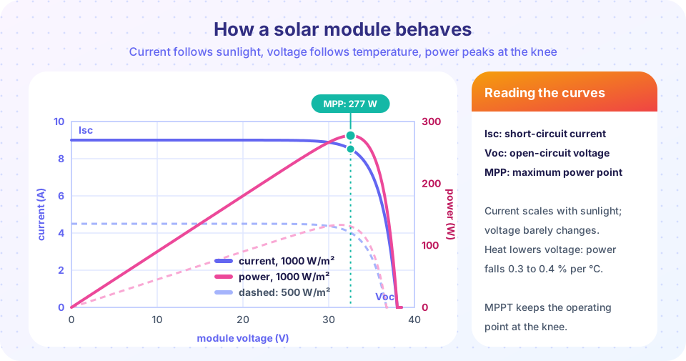
The curve has three landmark points: the short-circuit current Isc ≈ Iph at V = 0, the open-circuit voltage Voc ≈ a·ln(Iph/I0) at I = 0 (about 0.6 V per cell, 38 V for a 60-cell module), and the maximum power point (Vmp, Imp) at the knee, where V·I peaks. The ratio FF = Pmp/(Voc·Isc) measures the squareness of the curve. Because current is proportional to irradiance while the voltage depends only logarithmically on it, power is almost proportional to sunlight.
Efficiency is η = Pmp / (G·A). A 400 W module of area 1.95 m² under 1,000 W/m² has η = 400 / 1,950 = 20.5 %, typical of modern crystalline silicon.
Temperature
A hotter cell has a lower voltage: Voc falls by about 0.3 % per degree, while current rises only slightly. Net power drops by roughly 0.3 to 0.4 % per °C above 25 °C. On a hot day a cell can sit 25 to 30 °C above ambient, so a panel loses 10 % or more of its rated power in summer heat, and a panel in a cool, sunny climate can out-produce one in a desert.
MPPT
Because the MPP moves with sunlight and temperature, the inverter or a DC optimizer continuously searches for it. The classic perturb and observe algorithm nudges the voltage and keeps going in the direction that increases power; if power falls it reverses. A good algorithm tracks to within 1 % of the true maximum.
Annual energy
A fast estimate uses peak sun hours (the equivalent hours per day at 1,000 W/m²) and a performance ratio PR (0.75 to 0.85) that bundles temperature, wiring, dust and inverter losses:
E = P_rated × peak sun hours × 365 × PR
A 5 kW rooftop array in a location with 5 peak sun hours and PR = 0.8 produces 5 × 5 × 365 × 0.8 = 7,300 kWh per year, a capacity factor of 7,300 / (5 × 8,760) = 16.7 %.
How a wind turbine behaves
The kinetic power of air moving at speed v through a rotor of swept area A is ½·ρ·A·v³, with ρ = 1.225 kg/m³ at sea level (lower at altitude or in hot weather, since ρ = p/(R·T)). A turbine extracts a fraction Cp, the power coefficient:
P = ½ · ρ · A · v³ · Cp
Two consequences follow. First, the cube law: doubling the wind speed gives eight times the power, so a few extra meters per second at a site matter enormously. Second, the Betz limit: if the rotor extracted all the kinetic energy the air would stop behind it and block the flow, so the optimum is to slow the wind to one third of its upstream speed, giving Cp,max = 16/27 = 0.593. Real turbines reach Cp of 0.40 to 0.50.
Example: a rotor of diameter 120 m has A = π·60² = 11,310 m². In a 10 m/s wind with Cp = 0.45, P = 0.5 × 1.225 × 11,310 × 1000 × 0.45 = 3.12 MW.
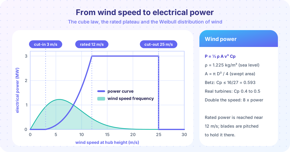
The power curve has four regions. Below the cut-in speed (about 3 m/s) the turbine does not run. Between cut-in and the rated speed (about 11 to 13 m/s) power follows the cubic rise as the controller keeps the tip-speed ratio (λ = ωR/v, around 7 to 9) at the value that maximizes Cp. From rated to cut-out (about 25 m/s) the blades are pitched to shed wind, holding power at the rated value. Above cut-out the rotor is stopped to protect it.
Large turbines use either a doubly fed induction generator with a partial-rated converter or a full-converter synchronous generator (often permanent magnet): both decouple the rotor speed from the grid frequency, which is why wind turbines add no natural inertia unless the control is designed to provide it (see the next lesson).
Wind statistics and capacity factor
Wind speeds at a site follow a Weibull distribution with density f(v) = (k/c)·(v/c)^(k−1)·exp(−(v/c)^k), where k (shape, about 2) and c (scale, a bit above the mean) are fitted to measurements; the mean is c·Γ(1 + 1/k). The expected power is the integral of the power curve times f(v), and the capacity factor is expected power divided by rated power. Site selection is largely a search for a large c.
Common misconceptions
"A 400 W panel produces 400 W." Only at STC. Real operation is lower in cloud, heat and dust: expect an annual average of roughly 15 to 20 % of rated power in a good location.
"The wind turbine runs at rated power most of the time." Wind speeds follow a distribution with a mean far below rated speed, so capacity factors of 25 to 45 % are normal.
"Betz limit is a design flaw." It is a physical limit for any rotor in an open flow; the best turbines already reach 75 to 85 % of it.
Try it
The first example implements the single-diode model with an irradiance and temperature correction, finds the maximum power point numerically and compares three conditions. It is an ideal-cell model (no series resistance), so the fill factor is a bit optimistic.
Press Run (or Ctrl + Enter) to see the result here.
Program input · what you'd type while the program runs
Type the answers before you press Run, one per line. Each time the program reads a line (with input()), it gets the next line from this box.
The second example combines a power curve with a Weibull wind distribution to get the capacity factor and annual energy of a 3 MW turbine at sites with different mean wind speeds.
Press Run (or Ctrl + Enter) to see the result here.
Program input · what you'd type while the program runs
Type the answers before you press Run, one per line. Each time the program reads a line (with input()), it gets the next line from this box.
The third example is a quick wind-power calculator. Change the rotor diameter, the wind speed and Cp; it shows the power and compares it with the Betz-limited maximum.
Check your understanding
Quick check · 5 questions
of 5 answered You scored / 5 · perfect!
-
1. A 300 W module has an area of 1.7 m2. What is its efficiency at STC (1000 W/m2)?
eta = 300 / (1000 x 1.7) = 0.176. -
2. What happens to a solar module's power when the cell temperature rises?
Voltage drops about 0.3 % per K while current rises only slightly. -
3. A wind turbine sees the wind speed rise from 6 to 12 m/s (same Cp, below rated). By what factor does power rise?
Power is proportional to v cubed: 2 cubed = 8. -
4. Which value is the Betz limit?
No rotor can capture more than 16/27 of the wind's kinetic power. -
5. A 4 kW rooftop PV system gets 4.5 peak sun hours per day with a performance ratio of 0.8. Annual energy is about
4 x 4.5 x 365 x 0.8 = 5,256 kWh.
Summary
- A PV module is a diode with a light-driven current:
Isc,Voc, fill factor and a maximum power point that MPPT tracks. - Power is nearly proportional to irradiance and falls about 0.3 to 0.4 % per degree of heating.
- Wind power is
½ρA·v³·CpwithCp ≤ 16/27; the cube law makes site wind speed the dominant factor. - Annual energy: PV from peak sun hours and performance ratio; wind from the power curve and a Weibull wind distribution.
- Typical capacity factors are 15 to 30 % (solar) and 25 to 45 % (onshore wind).
Track your progress
Create a free account to tick off lessons and pick up where you left off on any device.
of Electric Power Systems lessons completed