


















Lesson 37 of 47 · Smart Grids and Economics
Economic dispatch
Learn to share load among generators at least cost: cost curves, the equal incremental cost rule, lambda iteration with limits, penalty factors for losses and unit commitment.
Demand at a given moment is a number, say 700 MW. Dozens of generators could in principle supply it, and they do not all cost the same to run: an efficient combined-cycle gas plant burns less fuel per megawatt-hour than an old peaker. Economic dispatch (ED) answers the question: given the units that are already running, how much should each produce so that the total cost is minimal? It is the core calculation inside every energy management system and, in a different guise, the logic of the electricity market.
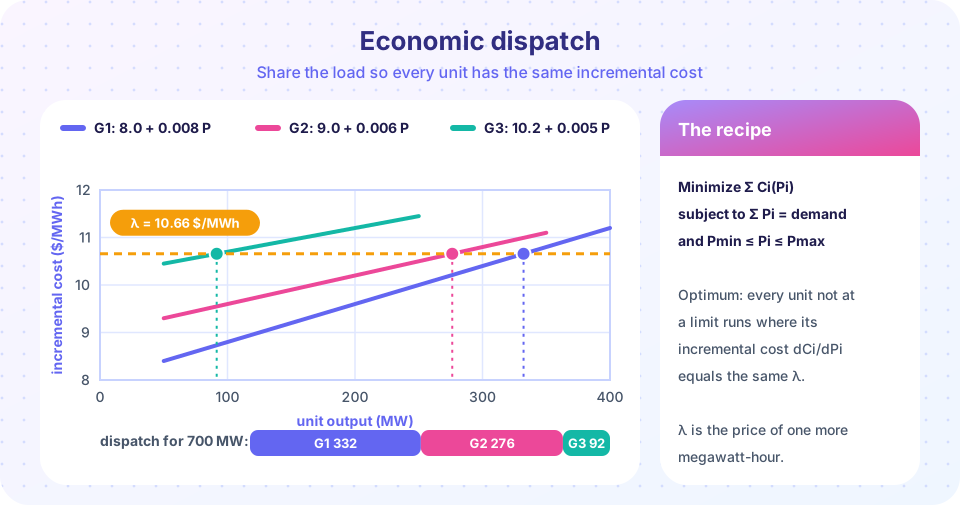
The answer is surprisingly elegant. At the optimum, all the units that are free to move run at the same incremental cost, and that common value λ is the price of one more megawatt-hour.
What you will learn
- Write a generator cost curve and its incremental cost.
- State and use the equal incremental cost rule, including generator limits.
- Solve a dispatch with lambda iteration.
- Account for transmission losses with penalty factors and see how unit commitment differs.
Key terms
Cost curve C(P): the cost per hour of producing power P, often C = a + b·P + c·P² in dollars per hour.
Incremental cost (IC): the cost of one more MWh, dC/dP = b + 2c·P.
Lambda (λ): the Lagrange multiplier of the demand constraint, equal to the system's marginal cost.
Penalty factor: a multiplier that makes a unit's cost reflect the extra losses it causes.
Unit commitment (UC): the decision of which units to run in each hour, before dispatch.
Cost curves
The fuel cost of a thermal unit is its fuel input (the heat rate times output) times the fuel price. Heat input rises faster than output because efficiency is best near rated power, so the cost curve is convex and usually fitted with a quadratic:
C(P) = a + b·P + c·P²          [$/h],   Pmin ≤ P ≤ Pmax
IC(P) = dC/dP = b + 2c·P       [$/MWh]
a covers the fixed cost of keeping the unit running at all; b is the linear fuel cost; c captures the loss in efficiency at high output. Because c > 0, the incremental cost increases with output: the more a unit produces, the more the next megawatt-hour costs. That is what makes sharing the load worthwhile. Two further pieces of data matter: the limits Pmin (below which a thermal unit cannot run stably) and Pmax, and, for realistic problems, ramp rates.
The equal incremental cost rule
Minimize the total cost ΣCi(Pi) subject to the power balance ΣPi = D. With a Lagrange multiplier,
L = Σ Ci(Pi) + λ·(D − Σ Pi) → dCi/dPi = λ for every unit
Intuition: if unit 1 had a lower incremental cost than unit 2, you could move one MW from 2 to 1 and reduce the cost, so you are not at the optimum. Only when all incremental costs are equal is there no improvement left.
Limits modify the rule (the Kuhn-Tucker conditions): units whose incremental cost at Pmax is still below λ are held at Pmax, those whose cost at Pmin is above λ are held at Pmin, and only the remaining units share the balance at equal IC.
Worked example
Three units supply 700 MW. Costs in $/h and limits in MW:
| Unit | Cost | Incremental cost | Limits |
|---|---|---|---|
| G1 | 120 + 8.0P + 0.004P² |
8.0 + 0.008P |
50 to 400 |
| G2 | 100 + 9.0P + 0.003P² |
9.0 + 0.006P |
50 to 350 |
| G3 | 80 + 10.2P + 0.0025P² |
10.2 + 0.005P |
50 to 250 |
Set Pi = (λ − bi)/(2ci): P1 = (λ − 8)/0.008, P2 = (λ − 9)/0.006, P3 = (λ − 10.2)/0.005. Their sum must equal 700:
λ·(125 + 166.67 + 200) = 700 + 1000 + 1500 + 2040
λ = 5,240 / 491.67 = 10.66 $/MWh
P1 = 332.2 MW,  P2 = 276.3 MW,  P3 = 91.5 MW     (sum 700)
All three lie inside their limits, so the answer is valid. At this λ the market price would be 10.66 $/MWh for every unit that moves.
Lambda iteration
For a general problem with limits there is no closed form, but the method is simple and robust: guess λ, compute each unit's output (clipped to its limits), compare the sum with the demand, adjust λ. A bisection search converges in a dozen iterations: if the total is too low raise λ, if too high lower it. Real systems with hundreds of units run this thousands of times a day.
Transmission losses and penalty factors
Power travelling over the network loses part of itself: typically 2 to 6 % of the energy. A unit far from the load causes more losses per MW than one next to it, so the cost of delivering a MW from that unit is higher than its fuel cost suggests. With loss PL(P1, ..., Pn) the balance is ΣPi = D + PL, and the optimum becomes
PFi · dCi/dPi = λ, PFi = 1 / (1 − ∂PL/∂Pi)
A unit that increases losses has ∂PL/∂Pi > 0, so its penalty factor exceeds 1 and it is dispatched less than a loss-free calculation would say. The third example below shows the effect. Modern markets build this into locational marginal prices (LMPs), where the price at each node contains an energy part, a loss part and a congestion part (next lesson).
Unit commitment
Dispatch assumes the units are already on. Unit commitment is the earlier, harder question of which units to start. A thermal unit takes hours to start, burns fuel to do so (start-up cost), must run at least a minimum time once on and stay off a minimum time once off, and has ramp limits. Committing too many units wastes fuel at minimum load; too few leaves the system short at the peak. UC is a mixed-integer optimization solved day-ahead for 24 to 168 hours, using techniques such as mixed-integer linear programming, with a rule-of-thumb "priority list" as the simplest approach (start the cheapest units first). Reserve margins and renewable forecast uncertainty are part of the constraints.
Common misconceptions
"Dispatch the cheapest unit first until it is full." That is the merit order, which is right when incremental costs are constant. With rising incremental costs, the optimum shares the load among units at equal IC.
"All units must run at the same output." They run at the same incremental cost, which usually means different outputs.
"λ is the average cost." λ is the marginal cost. It differs from average cost, which includes fixed costs.
Try it
The first example solves the dispatch with a bisection on λ that handles the limits, prints the 700 MW solution and compares its cost with a dispatch in proportion to the units' capacities.
Press Run (or Ctrl + Enter) to see the result here.
Program input · what you'd type while the program runs
Type the answers before you press Run, one per line. Each time the program reads a line (with input()), it gets the next line from this box.
The second example is the same dispatch in the browser: move the demand and watch the units share the load and lambda rise.
The third example adds losses. Two units serve 500 MW; unit 2 is remote and its flow causes losses PL = 0.0002·P2² (MW). The optimizer finds the dispatch for the lossless and the loss-aware problems. The lossless answer looks cheaper only because it forgets that about 15 MW of the output never reaches the customers.
Press Run (or Ctrl + Enter) to see the result here.
Program input · what you'd type while the program runs
Type the answers before you press Run, one per line. Each time the program reads a line (with input()), it gets the next line from this box.
Check your understanding
Quick check · 5 questions
of 5 answered You scored / 5 · perfect!
-
1. Two units both have IC1 = 20 and IC2 = 30 $/MWh at their present output. How can cost be reduced?
Producing one more MWh at unit 1 costs 20 and saves 30 at unit 2, a net gain of 10 $/MWh. -
2. A unit has C = 50 + 6P + 0.01P^2. What is its incremental cost at P = 100 MW?
IC = 6 + 2 x 0.01 x 100 = 8 $/MWh. -
3. What does lambda represent at the optimum?
Lambda is the marginal cost (the Lagrange multiplier of the demand constraint). -
4. A unit has penalty factor 1.05. Compared with a lossless dispatch, its output will be
Penalty factor above 1 raises the effective incremental cost, so the unit runs less. -
5. What does unit commitment decide?
UC chooses start-ups and shutdowns; dispatch then allocates output among the running units.
Summary
- Thermal cost curves are convex:
C = a + bP + cP²,IC = b + 2cP. - The optimum has equal incremental cost λ for all units not at a limit; units at a limit stay there.
- Lambda iteration solves it by bisection on λ.
- With losses, penalty factors
1/(1 − ∂PL/∂Pi)shift output away from units that cause more losses. - Unit commitment, a mixed-integer problem, decides which units run before dispatch allocates their output.
Track your progress
Create a free account to tick off lessons and pick up where you left off on any device.
of Electric Power Systems lessons completed