


















Lesson 8 of 47 · Generation and the Grid
Load Curves and Power Plants: Matching Supply to Demand
Read daily load curves and load duration curves, compute load factor and capacity factor, and see how a merit-order stack of plants meets demand at least cost.
Customers do not ask the power system politely. They flip switches whenever they like, and the generators must follow. The record of demand against time is the load curve. It is the most important picture in system planning, because it tells you how much capacity to build, which plant types to build and how they will be used.
What you will learn
- How to read a daily load curve and a load duration curve.
- How to compute load factor, capacity factor and related ratios.
- How base, intermediate and peaking plants fit the curve.
- How a merit-order dispatch picks plants and sets the price.
Key terms
- Load curve: demand (MW) against time, usually hourly over a day or a year.
- Load factor: average load divided by peak load over a period.
- Capacity factor: actual energy produced divided by the energy at full rated output for the whole period.
- Demand factor: maximum demand of a customer divided by its total connected load.
- Merit order: ranking of generators by marginal (running) cost, cheapest first.
The daily load curve
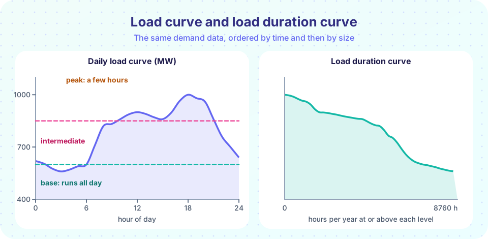
A typical weekday in a mild climate has a trough at night, a morning rise, a plateau through working hours and an evening peak when lighting, cooking and heating add to commercial load. Hot countries have an afternoon peak from air conditioning. Weekends are lower, and winter and summer differ. Planners study all of these by overlaying many days.
Three numbers summarize a day: the peak (maximum demand), the minimum and the average. Multiplying the average by 24 hours gives the energy consumed in MWh.
Load factor = average / peak. If the peak is 1000 MW and the day used 18,000 MWh, the average is 750 MW and the load factor is 75%. A high load factor means the capacity is used steadily; a low one means expensive equipment sits idle most of the time, which makes each kilowatt-hour dearer.
The load duration curve
Sort all 8760 hourly values of a year from largest to smallest and plot them with hours on the horizontal axis. The result is the load duration curve. It forgets when each level happened, but it shows how long each level lasted, which is what an investment decision needs.
- The area under the curve is the annual energy.
- The height at the left edge is the peak, present for only an hour or so.
- The height at the right edge is the minimum load, present all year: this is the baseload.
- Between them is a band of intermediate load and a spike of peak load.
If a power plant costs a lot to build but little to run, it should serve the flat, wide part of the curve. A plant that is cheap to build but expensive to run suits the narrow peak. That is the logic behind plant mix.
Capacity factor
For a plant of rated power Prated that produced energy E in a period T,
capacity factor = E / (Prated × T)
A 500 MW plant that produced 2,628,000 MWh in a year (8760 h) has 2,628,000 / (500 × 8760) = 60%. Typical capacity factors differ widely by plant type. Baseload nuclear plants may exceed 80%, peaking turbines may be under 10%, and wind and solar capacity factors depend on the site and the weather.
Do not confuse capacity factor (about one plant) with load factor (about the demand). Both are averages divided by maxima.
Merit-order dispatch
The operator wants to meet demand at the lowest total running cost. The rule is simple: line the plants up from cheapest marginal cost to dearest, and switch them on in that order until their combined output equals demand. The last plant used is the marginal unit. In many markets its cost sets the price paid to all plants in that hour.
Example for a demand of 900 MW (illustrative costs):
| Plant | Capacity (MW) | Cost ($/MWh) | Cumulative (MW) |
|---|---|---|---|
| Run-of-river hydro | 150 | 5 | 150 |
| Nuclear | 400 | 10 | 550 |
| Coal | 300 | 30 | 850 |
| Combined-cycle gas | 200 | 45 | 1050 |
| Gas peaker | 100 | 120 | 1150 |
At 900 MW, hydro, nuclear and coal run fully and gas runs at 50 MW, so gas is marginal. The running cost is 150×5 + 400×10 + 300×30 + 50×45 = $16,000 per hour. If all plants were paid the marginal price of $45, the payments would be 900 × 45 = $40,500, so cheaper plants earn a profit toward their capital costs.
Real dispatch adds constraints: ramp limits, minimum run levels, start-up costs, network limits and reserve requirements, which turn the problem into an optimization. Chapter 8 returns to it.
Common misconceptions
- "Peak demand is the average multiplied by a constant." The relation is the load factor, which changes with climate, industry and season.
- "A low capacity factor means a bad plant." A peaker is built to run rarely; its low capacity factor is by design, and its value lies in being available at the peak.
- "The grid needs capacity equal to the average load." It must cover the peak, plus reserve margin for outages.
Try it
First, compute the statistics of a synthetic daily curve and sort it into a duration curve. The 24 hourly values are illustrative, not from a real utility.
Press Run (or Ctrl + Enter) to see the result here.
Program input · what you'd type while the program runs
Type the answers before you press Run, one per line. Each time the program reads a line (with input()), it gets the next line from this box.
Second, run a merit-order dispatch. Change the demand in the code, run it again, and watch which plant becomes marginal.
Press Run (or Ctrl + Enter) to see the result here.
Program input · what you'd type while the program runs
Type the answers before you press Run, one per line. Each time the program reads a line (with input()), it gets the next line from this box.
Check your understanding
Quick check · 5 questions
of 5 answered You scored / 5 · perfect!
-
1. A system has a peak of 800 MW and consumes 14,400 MWh in a day. What is its load factor?
Average = 14,400 / 24 = 600 MW. Load factor = 600 / 800 = 75%. -
2. A 200 MW wind farm produces 438,000 MWh in a year. What is its capacity factor?
Full-output energy is 200 × 8760 = 1,752,000 MWh. 438,000 / 1,752,000 = 25%. -
3. What does the load duration curve discard?
Sorting by size removes the time order but keeps the durations and the total energy. -
4. In a merit-order dispatch, which plant runs first?
Cheapest running cost first minimizes the total cost of meeting demand. -
5. Why does a peaking plant have a low capacity factor yet still earn its place?
Low capital cost and fast starts make it the cheapest way to cover rare peaks.
Summary
- The load curve shows demand over time; the load duration curve sorts it to show how long each level lasts.
- Load factor
= average / peak; capacity factor= E / (Prated × T). - Baseload plants (cheap to run) serve the flat part of the duration curve; peakers serve the narrow top.
- Merit-order dispatch runs the cheapest plants first; the last one running is marginal.
- Real dispatch adds ramp, network and reserve constraints.
Next: Transformers
Track your progress
Create a free account to tick off lessons and pick up where you left off on any device.
of Electric Power Systems lessons completed