


















Lesson 15 of 47 · Transmission Lines
Chapter 3 Review: Transmission Lines
Review line parameters, short, medium and long line models, voltage regulation, the Ferranti effect and SIL with a poster, recap table, calculator and ten-question quiz.
Chapter 3 gave you the tools to turn a line, with its towers, conductors and spacing, into numbers and circuits. You learned to compute R, L and C from geometry, to pick a model by length, and to read a line's behavior through its characteristic impedance and surge impedance loading. This page ties them together.
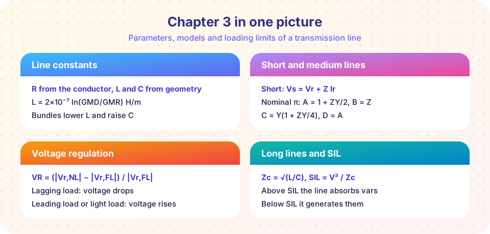
What you will review
- Line constants from GMD, GMR and bundling.
- Short, nominal-π and distributed models, and ABCD constants.
- Voltage regulation, the Ferranti effect and charging current.
- Characteristic impedance and surge impedance loading.
Recap table
| Topic | Key relations | Lesson |
|---|---|---|
| Inductance | L = 2×10⁻⁷ ln(GMD / Ds) H/m |
Line Parameters |
| Capacitance | C = 2π ε0 / ln(GMD / r) F/m |
Line Parameters |
| Bundle GMR (two conductors) | Ds,b = √(Ds d) |
Line Parameters |
| Short line | Vs = Vr + Z Ir |
Short and Medium Lines |
| Nominal π | A = 1 + ZY/2, B = Z, C = Y(1 + ZY/4), AD − BC = 1 |
Short and Medium Lines |
| Regulation | (Vr,NL − Vr,FL) / Vr,FL (magnitudes) |
Short and Medium Lines |
| Long line | Vs = Vr cosh γl + Zc Ir sinh γl |
Long Lines and Surge Impedance Loading |
| Ferranti | Vr = Vs / cos βl (open, lossless) |
Long Lines and Surge Impedance Loading |
| SIL | VLL² / Zc, Zc = √(L / C) |
Long Lines and Surge Impedance Loading |
Worked review example
A 230 kV, 80 km line has r = 0.07 Ω/km, L = 1.3 mH/km and C = 8.8 nF/km at 50 Hz. Classify it and find its key numbers.
- At 80 km it sits at the border of the short and medium ranges; the charging current is small, so a short-line model is acceptable for a first estimate.
- Reactance
x = 2π × 50 × 1.3×10⁻³ = 0.408 Ω/km, soZ = 5.6 + j32.7 Ω. - Characteristic impedance
Zc = √(1.3×10⁻³ / 8.8×10⁻⁹) = 384 Ω, soSIL = 230² / 384 = 138 MW. - Phase constant
β = 2π × 50 × √(LC) = 1.06×10⁻³ rad/km, soβl = 4.9°: the line is only a few degrees long, and the open-end Ferranti rise is under 1%.
Loading this line with 120 MW is close to SIL, so voltage will vary little along it. The Python block below completes the calculation with regulation and loss.
Common misconceptions
- "Use the longest model every time." The distributed model is exact but needs more work. A short line analyzed with the long model gives the same answer; use the simplest model that is accurate enough.
- "SIL depends on the line length."
Zcdepends on per-kilometer constants, so SIL does not change with length. - "The voltage at the end of a line always drops." With light load or a leading load, it can rise.
Try it
First, a toolkit that computes everything for the worked example. Change the load and the length at the top.
Press Run (or Ctrl + Enter) to see the result here.
Program input · what you'd type while the program runs
Type the answers before you press Run, one per line. Each time the program reads a line (with input()), it gets the next line from this box.
Second, flash cards for the key relations. Flip each card and rate yourself honestly.
Check your understanding
Quick check · 9 questions
of 9 answered You scored / 9 · perfect!
-
1. Which change lowers a line's reactance?
A bundle has a larger effective radius, which reduces L. Wider spacing and higher frequency raise reactance. -
2. Phases are 5 m, 5 m and 10 m apart. The GMD is:
GMD = (5 × 5 × 10)^(1/3) = 250^(1/3) = 6.30 m. -
3. For a nominal π, if Z = 10 + j50 Ω and Y = j0.0004 S, what is A?
ZY = (10 + j50)(j0.0004) = j0.004 − 0.02 = −0.02 + j0.004, so ZY/2 = −0.01 + j0.002 and A = 1 + ZY/2 = 0.99 + j0.002. -
4. A 500 kV line has Zc = 250 Ω. What is its SIL?
SIL = 500² / 250 = 1000 MW. -
5. On a lightly loaded long line, the receiving-end voltage is higher than the sending-end voltage because of:
Charging current flowing through the series inductance raises the voltage: the Ferranti effect. -
6. Which model would you choose for a 600 km overhead line?
Beyond about 250 km the lumped models lose accuracy; use the distributed model. -
7. A line loaded at exactly its SIL has what feature?
At SIL the reactive power produced by capacitance equals that absorbed by inductance, so the voltage profile is flat (for a lossless line). -
8. Heating an aluminum conductor from 20 °C to 70 °C raises its resistance by about:
α ≈ 0.004 per °C, so a 50 °C rise gives about +20%. -
9. Which has the larger capacitance per kilometer, an overhead line or an underground cable?
In a cable the conductors are close to the grounded sheath, so capacitance is much higher.
Summary
- Geometry fixes the line constants:
Lfromln(GMD / Ds),Cfromln(GMD / r); bundling lowersLand raisesC. - Short lines use series
Z; medium lines use a nominal π; long lines usecoshandsinhofγl. - Voltage regulation depends strongly on the load power factor; leading or light loads can raise voltage.
Zc = √(L / C)andSIL = VLL² / Zcsummarize a line's natural loading; the Ferranti rise is1 / cos βl.- Chapter 4 introduces the per-unit system and load-flow analysis for whole networks.
Track your progress
Create a free account to tick off lessons and pick up where you left off on any device.
of Electric Power Systems lessons completed