


















Lesson 38 of 47 · Smart Grids and Economics
Electricity markets and demand response
Learn how wholesale electricity markets clear with the merit order, how locational prices reveal congestion, how demand response lowers prices, and how to compare costs with LCOE.
Economic dispatch describes what a central planner would do with complete cost information. Most countries now use competitive electricity markets to arrive at nearly the same answer: generators submit offers, an independent operator clears them against demand, and a price emerges. The market is a mechanism for discovering costs and giving everyone, from a coal plant to a household water heater, a reason to do the efficient thing.
This lesson explains how the standard wholesale market clears, why prices differ from place to place, how flexible demand changes the outcome, and how engineers compare the cost of different technologies.
What you will learn
- Explain the merit order and uniform-price clearing.
- Describe day-ahead, real-time, ancillary and capacity markets.
- Understand locational marginal prices and congestion rent.
- Quantify what demand response does to prices and compare technologies with LCOE.
Key terms
Merit order: ranking of generators by increasing marginal cost.
Uniform price auction: every accepted generator is paid the price of the last (marginal) unit needed.
Locational marginal price (LMP): the cost of serving one more MW at a particular bus, including energy, losses and congestion.
Demand response (DR): customers reducing or shifting consumption in response to prices or signals.
LCOE: levelized cost of energy, the lifetime cost of a plant per MWh produced.
The merit order and the clearing price
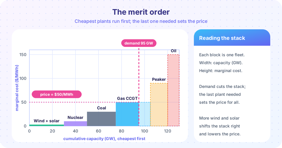
In a competitive market each generator offers energy at (roughly) its marginal cost: for a wind farm, near zero; for a gas plant, the fuel and variable O&M cost per MWh. The operator sorts the offers from cheapest to most expensive, builds up the supply curve, and stops where cumulative supply meets demand. The offer of the last unit needed sets the clearing price, and in a uniform-price market every generator that is accepted receives that price.
In the figure, demand of 95 GW needs wind and solar (30 GW at 0 $/MWh), nuclear (20 GW at 10), coal (25 GW at 30) and part of the combined-cycle fleet at 50 $/MWh, so the price is 50 $/MWh. Wind earns 50 for every MWh although it costs almost nothing to produce; the difference is inframarginal rent that pays for capital costs. Why pay everyone the marginal price? Because it gives each unit the right incentive: offer your true cost, as being lower than the price never loses money and a higher offer only risks being excluded.
When demand falls, a more expensive block is no longer needed and the price drops; when wind and solar grow, they push everything right along the curve and lower the price, the merit-order effect. At times when renewables alone exceed demand, prices can reach zero or even turn negative, because subsidized plants or inflexible units would rather pay than shut down.
Markets in time
- Day-ahead market: the operator clears hourly prices for the next day using offers and forecasts; it also decides which units to commit.
- Real-time (balancing) market: every 5 to 15 minutes the operator re-dispatches to cover forecast errors and outages. Participants who deviate from their day-ahead positions are paid or charged the real-time price.
- Ancillary services: frequency regulation, spinning and non-spinning reserves, voltage support and black-start capability are procured and paid separately.
- Capacity markets or mechanisms: payments for being available at the peak, in systems where energy prices alone may not recover the cost of rarely used peaking plant.
- Forward and bilateral contracts: most energy is hedged long before delivery; the spot market handles the remainder.
Locational marginal pricing and congestion
If the network had no limits, one price would serve the whole system. In reality lines have thermal limits, and when a cheap generator cannot send more power to a load pocket, the expensive local generator must run. The marginal cost of serving the next MW then depends on where it is delivered. The LMP at a bus is exactly that marginal cost; it is the Lagrange multiplier of the bus power balance in the optimal power flow, and it consists of three components:
LMP = energy component + loss component + congestion component
Example: two buses, A and B. Cheap generation at A costs 20 $/MWh, and expensive generation at B costs 60 $/MWh. The whole load, 150 MW, is at B, and the line A to B can carry 100 MW. The optimum runs 100 MW from A and 50 MW from B. The extra MW at B must come from B's 60 $/MWh unit (the line is full), so LMP_B = 60; an extra MW at A could be supplied by A's own generator at LMP_A = 20. The difference, 40 $/MWh times 100 MW = 4,000 $/h, is the congestion rent collected by the grid operator. It shows exactly how much a new line or a battery in the load pocket would be worth.
Demand response
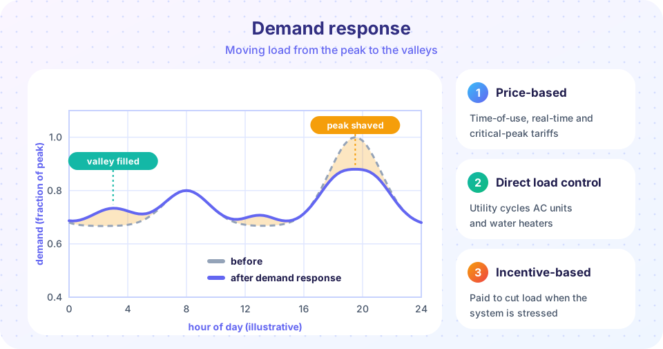
Demand has traditionally been treated as fixed, but customers have flexibility: thermostats, water heaters, industrial processes, electric vehicles, batteries. A demand response program pays customers or charges them time-varying prices to use less (or more) at certain hours. Its value comes from the shape of the supply curve: the last units are far more expensive than the first, so a small reduction of demand at the peak removes the costliest generator and lowers the price for everyone. In the merit order a demand of 125 GW is met by the oil block at 150 $/MWh. If DR removes 8 GW, the price falls to the peaker price of 90 $/MWh; consumers' total bill drops from 125 × 150 = 18,750 to 117 × 90 = 10,530 (thousand dollars per hour), far more than the cost of the demand response itself.
Types: price-based (time-of-use, critical-peak and real-time tariffs), direct load control (the utility cycles air conditioners), and incentive-based programs (interruptible loads, paid for the capacity to curtail). Short-run price elasticity is typically small (a few percent change in use per 10 % price change), so the volumes come from automation rather than from conscious behavior.
Comparing costs: LCOE
To compare technologies with different capital and fuel costs, planners use the levelized cost of energy, the constant price per MWh that would exactly repay all lifetime costs:
LCOE = ( Capex × CRF + Fixed O&M ) / (8,760 × CF)  +  Fuel cost + Variable O&M
CRF = r (1 + r)^n / ( (1 + r)^n − 1 )          (capital recovery factor)
where r is the discount rate and n the lifetime. With illustrative numbers, a solar plant at 1,000 $/kW, 25 % capacity factor, 15 $/kW-year fixed O&M, 25 years and 7 % gives CRF = 0.0858, (85.8 + 15)/2,190 = 46 $/MWh. A gas combined-cycle plant at 1,000 $/kW, 60 % capacity factor, 6.5 MMBtu/MWh at 4 $/MMBtu and 3 $/MWh variable O&M comes to about 47 $/MWh, but 55 % of it is fuel and exposed to gas prices.
LCOE is a useful but limited measure: it ignores when energy is produced (an MWh at noon is worth less than one in the evening), the cost of integration and the system value of firm capacity. For this reason system studies compare value-adjusted costs or run full market simulations.
Common misconceptions
"Uniform pricing overpays cheap generators." The inframarginal rent covers their fixed costs; with pay-as-bid, generators would offer higher and strategize, and the clearing would not reveal true costs.
"Renewables always lower consumers' bills." They lower the wholesale price in the hours they run (merit-order effect), but the cost of network, balancing and any subsidies also reaches consumers.
"LCOE says everything." It misses timing, integration costs and reliability; two plants with the same LCOE can have very different values to the grid.
Try it
The first example clears the merit order from the figure for different demands, shows what extra wind and solar do to the price, and computes the effect of an 8 GW demand response at a peak. It is a stylized stack, not market data.
Press Run (or Ctrl + Enter) to see the result here.
Program input · what you'd type while the program runs
Type the answers before you press Run, one per line. Each time the program reads a line (with input()), it gets the next line from this box.
The second example computes locational marginal prices for the two-bus example with a linear program. The shadow prices of the bus balances are the LMPs.
Press Run (or Ctrl + Enter) to see the result here.
Program input · what you'd type while the program runs
Type the answers before you press Run, one per line. Each time the program reads a line (with input()), it gets the next line from this box.
The third example is an LCOE calculator with illustrative inputs. Change the capital cost, the capacity factor, the discount rate and the fuel cost.
Check your understanding
Quick check · 5 questions
of 5 answered You scored / 5 · perfect!
-
1. In a uniform-price market, what price do all accepted generators receive?
The clearing price is set by the last unit needed; all accepted units are paid it. -
2. What does the merit-order effect describe?
Adding cheap supply shifts the merit order and lowers the clearing price in the hours it runs. -
3. LMP at the load bus is 60 $/MWh and at the generator bus 20 $/MWh with 100 MW flowing. What is the congestion rent per hour?
(60 - 20) x 100 = 4,000 dollars per hour. -
4. Why does a small amount of demand response lower prices so much at the peak?
Supply curves are steep at the peak, so a small reduction of demand cuts the marginal cost sharply. -
5. A plant costs 2,000 $/kW, has CRF = 0.08 and fixed O&M of 40 $/kW-year, with CF = 50 % and no fuel. Its LCOE is about
(2,000 x 0.08 + 40) / (8.76 x 0.5) = 200 / 4.38 = 45.7 dollars per MWh.
Summary
- Markets sort offers into a merit order and clear at the marginal unit's price; inframarginal plants earn rent.
- Day-ahead, real-time, ancillary and capacity markets cover energy, balancing, reserves and availability.
- LMPs include energy, loss and congestion components; congestion separates prices and creates rent.
- Demand response removes the costliest generation at the peak and lowers prices for everyone.
- LCOE = (Capex × CRF + fixed O&M)/(8,760 × CF) + variable cost; useful but blind to timing and integration cost.
Track your progress
Create a free account to tick off lessons and pick up where you left off on any device.
of Electric Power Systems lessons completed