


















Lesson 18 of 47 · Per-Unit Analysis and Load Flow
The Bus Admittance Matrix (Ybus) and Power Injections
Build the bus admittance matrix Ybus of a power network by inspection, understand its properties, and use it to compute bus power injections and line flows.
If a power network has a few buses you can solve it with series and parallel reductions. With hundreds or thousands of buses you need a systematic method. Nodal analysis gives one: write Kirchhoff's current law at every bus and collect the results in a matrix. That matrix, the bus admittance matrix Ybus, is the data structure at the center of load flow, fault analysis and stability studies. This lesson shows how to build it by inspection and how to use it to compute power.
What you will learn
- How nodal equations lead to
I = Ybus V. - The rules for filling
Ybusby inspection, including shunt elements. - Properties of
Ybus: symmetry, sparsity and singularity. - How to get bus power injections and line flows from voltages.
Key terms
- Admittance (y): the reciprocal of impedance,
y = 1/z = g + jb, in siemens or per-unit. - Self-admittance (Yii): the diagonal entry for bus
i. - Mutual admittance (Yij): the off-diagonal entry between buses
iandj. - Injection: the current or power entering the network at a bus.
- Sparse matrix: a matrix with mostly zero entries, typical of large networks.
From Kirchhoff to a matrix
Number the buses 1 to n and pick a ground reference. Let Vi be the voltage of bus i with respect to ground and Ii the current injected into bus i from outside (a generator or a load, with sign). Kirchhoff's current law at each bus says the injection equals the sum of currents leaving through branches. For a line with admittance yij between buses i and j, the current leaving i is yij (Vi − Vj). Collecting terms:
Ii = (Σj yij) Vi − Σj yij Vj
for every bus, which is the matrix equation
I = Ybus × V
with:
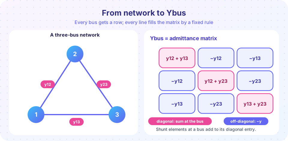
Yii = Σ (all admittances connected to bus i), including any shunt admittanceyi0to ground;Yij = −yij(negative of the admittance directly connectingiandj), and0if no line connects them.
That is the whole procedure: go through the buses, add the admittances meeting at each one on the diagonal, and put the negative of each branch admittance in the matching off-diagonal positions. Per-unit values are used so that transformers (with their per-unit impedances) and lines at different voltage levels live in the same matrix.
Worked example: three buses
Take the triangle in the picture, in per-unit on a 100 MVA base, with line impedances
z12 = 0.02 + j0.06, z13 = 0.04 + j0.12, z23 = 0.03 + j0.09.
The admittances are y12 = 1/z12 = 5 − j15, y13 = 2.5 − j7.5 and y23 = 3.333 − j10. Then
Y11 = y12 + y13 = 7.5 − j22.5Y22 = y12 + y23 = 8.333 − j25Y33 = y13 + y23 = 5.833 − j17.5Y12 = Y21 = −y12 = −5 + j15,Y13 = Y31 = −2.5 + j7.5,Y23 = Y32 = −3.333 + j10
So the matrix, in per-unit siemens, is
| Bus 1 | Bus 2 | Bus 3 | |
|---|---|---|---|
| Bus 1 | 7.5 − j22.5 | −5 + j15 | −2.5 + j7.5 |
| Bus 2 | −5 + j15 | 8.333 − j25 | −3.333 + j10 |
| Bus 3 | −2.5 + j7.5 | −3.333 + j10 | 5.833 − j17.5 |
Properties
- Symmetric (
Yij = Yji) when there are no phase-shifting transformers: the network is reciprocal. - Sparse: a bus connects to only a few others. In a real network with thousands of buses, over 99% of the entries are zero, and software stores only the non-zero ones.
- Singular when there are no shunts to ground: each row sums to zero (check the example:
7.5 − 5 − 2.5 = 0). Without a reference you cannot find absolute voltages; in load flow the slack bus fixes the reference. - Line charging enters as shunt terms. A line with total charging susceptance
BaddsjB/2to the diagonal of each of its end buses, as in the π model.
Transformers with an off-nominal tap a (a ratio other than 1 per unit) need modified entries: the Yii on the tapped side becomes y / a² and the mutual terms become −y / a. Phase shifters make the matrix non-symmetric. Those details matter in practice but the principle is unchanged.
Power injections
The complex power injected at bus i is Si = Vi Ii* = Pi + jQi. Substituting Ii = Σj Yij Vj gives the power-flow equations:
Pi = Σj |Vi||Vj| (Gij cos θij + Bij sin θij)
Qi = Σj |Vi||Vj| (Gij sin θij − Bij cos θij)
where Yij = Gij + jBij and θij = δi − δj. Given every voltage magnitude and angle, these formulas give the power at every bus directly. In load flow the problem runs the other way: powers are specified and voltages are unknown, so these equations are solved iteratively (next lesson).
Line flows follow from branch currents. For the line from i to j, Sij = Vi (Vi − Vj)* yij* plus the charging term if present. The power lost in the line is Sij + Sji.
Numbers for the example
Suppose the voltages are V1 = 1.04∠0°, V2 = 1.00∠−2° and V3 = 0.98∠−4°. Then I = Ybus V and S = V × conj(I) give
- Bus 1:
S1 = 1.451 + j0.761 pu(generating) - Bus 2:
S2 = −0.331 − j0.317 pu(a load) - Bus 3:
S3 = −1.079 − j0.321 pu(a larger load)
The sum 0.041 + j0.123 pu is the total network loss (4.1 MW and 12.3 Mvar on a 100 MVA base). The reactive loss is larger than the real loss because the lines are mostly reactive, an important feature of transmission networks that you will see again in chapter 6.
Common misconceptions
- "Ybus is the inverse of the impedance matrix, so it needs inversion."
Ybusis built directly from branch admittances, with no inversion. Its inverseZbusis only needed for some fault studies. - "Off-diagonal entries are positive admittances." They are negative:
Yij = −yij. - "A line with no connection has infinite impedance, so I put a large number in Ybus." A missing line simply leaves a zero entry.
Try it
First, a general Ybus builder. It takes a list of lines, builds the matrix, checks that the row sums are zero (no shunts), and computes the injections for given voltages.
Press Run (or Ctrl + Enter) to see the result here.
Program input · what you'd type while the program runs
Type the answers before you press Run, one per line. Each time the program reads a line (with input()), it gets the next line from this box.
Second, an interactive builder. Change the resistance and reactance of each line and watch the matrix update. It prints each entry as G + jB. Notice that the row sums stay at zero.
Check your understanding
Quick check · 5 questions
of 5 answered You scored / 5 · perfect!
-
1. Bus 1 connects to bus 2 through y12 = 4 − j8 and to bus 3 through y13 = 2 − j4. What is Y11?
The diagonal entry is the sum of admittances connected to the bus: (4 − j8) + (2 − j4) = 6 − j12. -
2. What is Y12 in the same network?
Off-diagonal entries are the negative of the connecting admittance: −y12 = −4 + j8. -
3. Why is Ybus of a network with no shunt elements singular?
With no connection to ground, adding a constant to all bus voltages changes no current; the matrix has no unique solution. -
4. Buses 4 and 5 are not connected by any line. What is Y45?
No direct branch means a zero entry. -
5. How does line charging enter Ybus?
The π model puts half the line's shunt admittance at each end, adding to the diagonal entries.
Summary
I = Ybus V, withYiithe sum of admittances at busiandYij = −yij.- Ybus is sparse and (without phase shifters) symmetric; without shunts its rows sum to zero.
- Line charging and shunts add to the diagonal; off-nominal taps modify entries.
- Power injections:
Si = Vi (Σj Yij Vj)*, or thePiandQisums withGij,Bij,θij. - Given voltages these give powers directly; load flow solves the reverse problem iteratively.
Next: Newton-Raphson Load Flow
Track your progress
Create a free account to tick off lessons and pick up where you left off on any device.
of Electric Power Systems lessons completed