


















Lesson 20 of 47 · Structure and Properties
Viscoelasticity, creep and melt rheology
Learn why polymers are both solid and liquid, model them with springs and dashpots, apply the Deborah number, time-temperature superposition (WLF) and melt viscosity scaling.
Silly Putty bounces like a ball when you drop it and flows into a puddle if you leave it on a table overnight. A plastic shelf holds books for a week without a visible change and sags after a year. A rubber band lightly stretched for months does not return fully to its original length. These are not curiosities: they are the normal behavior of polymers, which are viscoelastic: part elastic solid and part viscous liquid. Which side you see depends on how fast you look. This lesson gives you the models and the vocabulary to describe it, from the springs and dashpots of the simplest theory to the equations engineers use to predict long-term behavior from short tests.
What you will learn
- What viscoelasticity means, and how creep and stress relaxation show it
- The Maxwell and Kelvin–Voigt models and their time constants
- How the Deborah number links the time scale of a material to the time scale of observation
- How time-temperature superposition and the WLF equation trade time for temperature
- How melt viscosity depends on shear rate and molar mass, and why dynamic mechanical analysis is useful
Key terms
Viscoelastic: showing both elastic (recoverable) and viscous (flowing) response.
Creep: slow increase of strain under a constant stress.
Stress relaxation: slow decrease of stress under a constant strain.
Relaxation time (τ): characteristic time of the material's response.
Storage modulus E′ and loss modulus E″: the elastic and viscous contributions to the response to an oscillating load.
Two ideal behaviors
An ideal elastic solid obeys Hooke's law, σ = Eε: stress depends only on strain, energy is stored and fully returned. An ideal viscous liquid obeys Newton's law, σ = η dε/dt: stress depends on the rate of strain, and energy is dissipated as heat. Steel at small strain is nearly elastic; water is nearly viscous. A polymer is between the two, and which side dominates depends on time and temperature.
Two experiments reveal it directly:
- Creep: apply a constant stress and watch the strain grow with time.
- Stress relaxation: stretch to a fixed strain and watch the stress decay.
A hot-dog-shaped rubber stretched and held shows the stress falling off, because chains slowly slide and entanglements release.
Spring-and-dashpot models
Engineers picture a polymer as a combination of springs (modulus E, elastic) and dashpots (a piston in a viscous fluid, viscosity η, viscous).
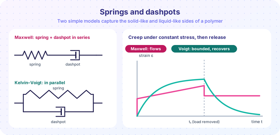
Maxwell model: spring and dashpot in series. Under a constant strain, the stress relaxes exponentially:
σ(t) = σ₀ exp(−t/τ) with τ = η/E.
Under constant stress, the strain jumps instantly (the spring) and then keeps growing linearly (the dashpot): the material flows. A Maxwell element is a model of a liquid with elastic memory, a melt or a lightly entangled polymer solution. If E = 1 MPa and η = 10⁶ Pa·s, τ = 1 second.
Kelvin–Voigt model: spring and dashpot in parallel. Under constant stress σ₀ the strain rises gradually toward a limit:
ε(t) = (σ₀/E)(1 − exp(−t/τ)), with τ = η/E,
and when the stress is removed the strain recovers exponentially to zero. It models a solid with delayed elasticity, like a crosslinked rubber.
Real polymers need several elements (the four-element Burgers model has an instantaneous elastic strain, a delayed elastic strain and viscous flow) or a whole spectrum of relaxation times, since chains of different lengths and segments of different sizes relax at different rates. Linear viscoelasticity assumes that stress responses simply add: the Boltzmann superposition principle lets you predict the response to any loading history from the response to a step.
The Deborah number
The Israeli-American rheologist Markus Reiner proposed the Deborah number, De = τ / t_obs, the ratio of the material's relaxation time to the observation (or experiment) time. The name comes from the prophetess Deborah's song in the Bible, "The mountains flowed before the Lord", meaning everything flows if you wait long enough. If De is large (a fast experiment or slow material), the material appears solid: Silly Putty bounces. If De is small (a slow experiment or fast relaxation), it appears liquid: Silly Putty flows on the table. The same material is both. This is why a polymer can shatter under a hammer yet creep slowly under a steady load.
Time-temperature superposition
Raising the temperature speeds up molecular motion. For polymers above Tg this speed-up is dramatic, and it is described by one factor: all relaxation times shrink by the same factor aT when you heat from a reference temperature Tr to T. A curve measured at a higher temperature is the same as the curve at the reference temperature viewed with a shifted time axis. By measuring at several temperatures over a modest time window and shifting the curves horizontally, you can build a master curve covering many decades of time: weeks, years or microseconds of behavior from a few hours of testing. This is how engineers predict creep over decades.
The shift factor is given by the Williams–Landel–Ferry (WLF) equation:
log₁₀ aT = −C₁ (T − Tr) / (C₂ + T − Tr).
With Tr = Tg, the "universal" constants for many amorphous polymers are about C₁ = 17.44 and C₂ = 51.6 K. At 20 K above Tg, log aT = −17.44 × 20/71.6 = −4.87, so relaxation is about 70,000 times faster. At 50 K above Tg it is about 10⁸ times faster. This explains why a polymer is glassy at Tg − 10 K and leathery or rubbery at Tg + 20 K.
Dynamic mechanical analysis
In dynamic mechanical analysis (DMA) a small sinusoidal strain is applied at frequency ω while the temperature changes. The stress response has two components: one in phase with the strain, the storage modulus E′ (elastic, energy stored) and one a quarter cycle out of phase, the loss modulus E″ (viscous, energy dissipated). Their ratio is tan δ = E″/E′. On heating through Tg, E′ drops by about three decades, E″ peaks and tan δ peaks at a temperature often reported as Tg. DMA also shows secondary transitions below Tg (local side-group motions), which govern low-temperature toughness. Because a high tan δ means energy is dissipated, polymers with a tan δ peak near the use temperature make good vibration dampers and shock absorbers; those with a low tan δ, like rubbers in tires designed for low rolling resistance, waste less energy.
Melt rheology
Processing means making a polymer flow. Polymer melts are non-Newtonian: viscosity is not a constant.
- Shear thinning. At low shear rates viscosity levels off at the zero-shear viscosity η₀; at high rates it falls, because chains disentangle and align with the flow. Over the range of shear rates in injection molding (10³ to 10⁵ s⁻¹) viscosity can drop by factors of 10 to 1,000 relative to η₀. In the power-law region,
η = K γ̇^(n−1)with n below 1. - Typical magnitudes. Melt viscosities of polymers at processing temperature are about 10² to 10⁵ Pa·s, compared with 10⁻³ Pa·s for water.
- Molar mass dependence. Below a critical molar mass Mc, chains are too short to entangle and
η₀ ∝ M. Above Mc, entanglements dominate andη₀ ∝ M^3.4(close to the 3.4 predicted by the reptation model of de Gennes, which pictures a chain wriggling like a snake in a tube formed by its neighbors, with corrections that give 3.4 instead of 3). For polystyrene Mc is about 35,000 g/mol, for polyethylene a few thousand. Doubling M above Mc increases η₀ about tenfold. - Elastic effects. Melts are also elastic: extrudate swells after leaving the die (die swell) and sharkskin roughness appears at high output rates.
Processing temperature, chain length and shear rate are chosen together: a high-molar-mass polymer has superb solid-state properties but is hard to process; manufacturers pick a molar mass compromise and use broad distributions.
Common misconceptions
"Glass is a liquid that flows over centuries." Ordinary window glass does not flow measurably; the uneven old panes come from how they were made. Polymers above Tg, however, do flow, which is why Tg matters.
"A polymer is either elastic or viscous." It is both, and the Deborah number says which dominates for a given observation time.
"Heating only softens a polymer a little." Above Tg a 20 K rise can speed up relaxation by a factor of tens of thousands, according to the WLF equation.
Try it
The first program plots stress relaxation of a Maxwell element, creep of a Kelvin–Voigt element and a table of Deborah numbers for the same material at different observation times. The second plots the WLF shift factor and the melt viscosity scaling with molar mass. All are idealized models with illustrative constants.
Press Run (or Ctrl + Enter) to see the result here.
Program input · what you'd type while the program runs
Type the answers before you press Run, one per line. Each time the program reads a line (with input()), it gets the next line from this box.
Press Run (or Ctrl + Enter) to see the result here.
Program input · what you'd type while the program runs
Type the answers before you press Run, one per line. Each time the program reads a line (with input()), it gets the next line from this box.
Check your understanding
Quick check · 5 questions
of 5 answered You scored / 5 · perfect!
-
1. A Maxwell element has E = 2 MPa and η = 4 × 10⁶ Pa·s. What is its relaxation time?
τ = η/E = 4 × 10⁶ / 2 × 10⁶ = 2 s. -
2. A material with De much greater than 1 behaves like
When the observation is much faster than relaxation, there is no time to flow, so it looks elastic. -
3. Which model describes delayed elasticity with full recovery and a limiting strain under constant stress?
The Kelvin–Voigt element approaches ε = σ₀/E and recovers fully when unloaded. -
4. What does time-temperature superposition allow?
Curves at different temperatures can be shifted along the time axis to form a master curve. -
5. Above the entanglement threshold, doubling the molar mass multiplies η₀ by roughly
η₀ ∝ M^3.4, and 2^3.4 ≈ 10.6.
Summary
- Polymers are viscoelastic: creep and stress relaxation show elastic and viscous behavior together, and the Deborah number
De = τ/t_obsdecides which one you see. - Maxwell (series) and Kelvin–Voigt (parallel) elements model flow and delayed elasticity, with
τ = η/E. - The WLF equation trades time for temperature above Tg; DMA measures E′, E″ and tan δ.
- Melts shear-thin, and above the entanglement threshold
η₀ ∝ M^3.4.
Next: Chapter 4 review
Track your progress
Create a free account to tick off lessons and pick up where you left off on any device.
of Polymer and Materials Chemistry lessons completed