


















Lesson 2 of 49 · Getting Started
What is econometrics?
Learn what econometrics is, how economic theory, data and statistics combine, the difference between prediction and causation, and the workflow of an analysis.
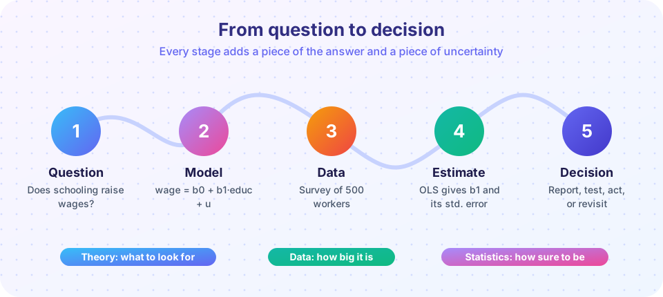
Economic theory is full of claims: demand curves slope downward, schooling raises productivity, higher interest rates cool inflation. Theory usually tells you the direction of an effect. It rarely tells you the size, and size is what decisions depend on. A central bank does not need to know that raising rates reduces inflation; it needs to know by how much, how quickly, and with what uncertainty. Econometrics measures economic relationships using data and statistical reasoning.
The word was coined in the early twentieth century, and the field took off in the 1930s with the founding of the Econometric Society. Ragnar Frisch, who introduced the term and shared the first Nobel Memorial Prize in Economic Sciences in 1969, argued that economics needed to unite theory, observation and mathematics. That three-way marriage is still the core of the subject.
What you will learn
- What econometrics is and what its three ingredients are.
- The difference between description, prediction and causal inference.
- How a real analysis moves from question to decision.
- Why economic data are harder to learn from than lab data.
Key terms
Parameter: an unknown number in the model, such as the true effect of schooling on wages.
Estimator: a recipe that turns data into a guess for a parameter. The number it produces is an estimate.
Disturbance (error term): everything that affects the outcome but is not in the model, written u.
Observational data: data recorded from the world as it happened, without the researcher assigning who gets what.
Counterfactual: what would have happened under a different choice.
Three ingredients
Economic theory supplies the question and the structure. It tells you that the quantity bought depends on price, income and tastes, so those belong in your equation, and it suggests signs: a higher price should reduce quantity.
Data supply the facts: prices, quantities, wages, years of schooling, firm sizes, interest rates, recorded across people, places or times.
Statistics supplies the machinery for learning from imperfect data: averages, regression, probability, hypothesis tests. Statistics tells you how much your estimate would bounce around if you drew a different sample.
Remove any one ingredient and the project fails. Theory without data is speculation. Data without theory is a pile of numbers you do not know how to interpret. Both without statistics give you an estimate and no idea how much to trust it.
A model is a purposeful simplification
An econometric model is an equation that says how an outcome is generated. A classic example links the hourly wage of a worker to years of schooling:
wage = β0 + β1 · educ + u
Here β0 (beta-zero) and β1 (beta-one) are the unknown parameters, educ is years of schooling and u is the disturbance that contains everything else: ability, experience, family connections, luck, the city a person lives in. The parameter β1 is the number we want, the dollars per hour that go with one more year of schooling.
The model is deliberately wrong in the sense that it leaves out most of life. All models do. The question is whether it is wrong in a harmless way. A map that omits every tree is fine for driving and useless for hiking; the right level of detail depends on the purpose. A good econometrician states clearly what is being left in u and argues why leaving it there is acceptable.
Worked example: reading the model
Suppose someone estimates β1 = 1.1 and β0 = 3 (the numbers in the previous lesson's invented data). Then the model predicts a wage of 3 + 1.1 × 16 = 20.6 dollars per hour for a worker with 16 years of schooling, and 3 + 1.1 × 12 = 16.2 for 12 years. The difference, 4.4 dollars, is four years times 1.1. The intercept β0 = 3 would be the prediction for zero years of schooling, which is an extrapolation far beyond the data: few workers have zero years of school, so do not take that number literally.
Three kinds of questions
It pays to be explicit about which question you ask, because each needs different evidence.
| Question type | Example | What you need |
|---|---|---|
| Description | What is the average wage of workers with a degree? | Representative data and a careful summary |
| Prediction | What wage will this applicant probably earn? | A model that forecasts well on new data |
| Causation | What would this person earn if she had one more year of schooling? | A research design that isolates the effect |
Description and prediction can be done well with a regression and large data. Causal questions are harder because the answer is a counterfactual: we observe a person with 12 years of schooling and a wage, but never the wage the same person would have had with 16 years. Chapter 6 and Chapter 8 are about designs that approximate that missing comparison.
Why economic data are difficult
A chemist can run an experiment: put identical samples in two flasks, change one thing, compare. Economists mostly cannot. You cannot randomly assign people to different levels of schooling, or countries to different interest rates. Instead we observe what happened, and what happened was the result of choices.
That creates the core difficulty of the field. People who choose more schooling differ from those who choose less in motivation, family background and ability. If you compare their wages you mix the effect of schooling with the effect of these other differences. Statisticians call such a mixing-up confounding; it is why "correlation is not causation" is the most repeated sentence in the subject.
Other difficulties follow. Data are noisy: measures contain errors. They are dependent: today's inflation is related to yesterday's, and neighbors affect each other. They are often limited: you have one history of the economy, not a thousand replays. A large share of the course teaches you to reason about these problems rather than to ignore them.
Fortunately there are also real tools. Randomized experiments are increasingly run in development economics, tech companies and labor studies. Natural experiments (a lottery, a sudden law change, a border that splits similar neighbors) mimic randomization. Econometric methods such as instrumental variables, difference-in-differences and regression discontinuity, which fill Chapters 6 and 8, exist to exploit these situations.
A real workflow
A responsible analysis follows a loop, not a line:
- Ask a precise question. "Does schooling matter?" is too vague. "By how many percent do hourly wages rise with one more year of schooling among full-time workers aged 25 to 54?" is precise.
- Connect it to theory. Which variables belong in the model? What sign do you expect? What could confound the relationship?
- Get and inspect the data. Where did they come from? Who is missing? How were variables defined? Plot before you model.
- Specify and estimate. Choose a functional form and an estimator. Record why.
- Check and challenge. Do the assumptions hold? Are results robust to reasonable changes? Does anything look odd?
- Interpret and communicate. Say what the estimate means, how precise it is, and what it cannot tell you.
Steps 5 and 6 are the ones beginners skip. Resist that temptation.
Common misconceptions
"A model is only useful if it is realistic in every detail." A model should be as simple as possible for its purpose. Extra realism often adds noise, not understanding.
"If my regression fits well, it proves the theory." A high fit means the model describes the sample. Several different theories can produce the same fit, so fit alone cannot tell them apart.
"Econometrics only uses regression." Regression is the workhorse, but the field also includes instrumental variables, panel methods, time series, nonlinear models for binary outcomes and many design-based methods.
Try it
First, a tiny experiment that shows why the error term matters. We generate two different samples from the same invented wage rule and compare the estimated slopes. They differ even though the true slope is identical. That sample-to-sample variation is the fundamental reason we need statistics.
Press Run (or Ctrl + Enter) to see the result here.
Program input · what you'd type while the program runs
Type the answers before you press Run, one per line. Each time the program reads a line (with input()), it gets the next line from this box.
Now a counterfactual illustration with invented numbers. Each person has two potential wages, one if they go to university and one if they do not. Real data show only one of the two. Because we simulate, we can see both and compare the true average effect with a naive comparison of the groups.
Press Run (or Ctrl + Enter) to see the result here.
Program input · what you'd type while the program runs
Type the answers before you press Run, one per line. Each time the program reads a line (with input()), it gets the next line from this box.
The naive gap exceeds the true effect because the groups differ in ability, not only in degrees. This is exactly the confounding problem described above, and fixing it is a recurring theme.
Check your understanding
Quick check · 5 questions
of 5 answered You scored / 5 · perfect!
-
1. Which three ingredients combine in econometrics?
Theory provides the question and structure, data provide the facts and statistics provides the tools for learning under uncertainty. -
2. In wage = β0 + β1·educ + u, what does u represent?
The disturbance collects everything else that affects wages: ability, experience, luck and so on. -
3. Why is a causal question harder to answer than a descriptive one?
The counterfactual outcome is missing, so a research design must stand in for it. -
4. A comparison of degree holders and non-holders overstates the effect of the degree because
This is confounding: the groups differ in other things that also affect wages. -
5. Which is a prediction question?
Prediction asks what value to expect for new data; causation asks what would change under an intervention.
Summary
- Econometrics measures economic relationships by combining theory, data and statistics.
- A model such as
wage = β0 + β1·educ + uis a purposeful simplification;uholds everything left out. - Distinguish description, prediction and causal questions; causal ones need a counterfactual.
- Economic data are observational, noisy and dependent, so confounding is the core challenge.
- A good analysis is a loop: question, theory, data, estimation, checking and communication.
Next: Data types and variables
Track your progress
Create a free account to tick off lessons and pick up where you left off on any device.
of Econometrics lessons completed