


















Lesson 9 of 49 · Data and the Regression Idea
Estimators and sampling distributions
Learn what an estimator is, why estimates vary from sample to sample, how to judge estimators by bias, variance and consistency, and what a standard error measures.
You never see the population. You see a sample: 500 workers out of millions, 40 quarters of a country's history. Yet the questions you care about concern the population: the true average wage, the true effect of schooling. So everything you compute from a sample is a guess at something you cannot observe. Econometrics gets its power, and its humility, from studying how good such guesses are.
The key insight of this lesson is a surprising one. Because a sample is random, an estimate is itself a random variable. If you could redo the survey with different people, you would obtain a different number. The distribution of those numbers across repeated samples is the sampling distribution, and almost everything we say about precision, tests and confidence intervals is a statement about it.
What you will learn
- The difference between a parameter, an estimator and an estimate.
- How to judge an estimator: bias, variance, mean squared error and consistency.
- What the law of large numbers and the central limit theorem say.
- What a standard error is and how it shrinks with sample size.
Key terms
Parameter: a fixed, unknown feature of the population, such as its mean μ.
Estimator: a rule that maps a sample to a number, such as the sample mean.
Estimate: the number the rule produces for one particular sample.
Sampling distribution: the distribution of an estimator over all possible samples of a given size.
Standard error: the standard deviation of an estimator's sampling distribution (or its estimate from data).
Parameter, estimator, estimate
Take the population average wage μ. This is a parameter: one fixed number, unknown to you. The sample mean
X̄ = (X1 + X2 + ... + Xn) / n
is an estimator: a recipe applied to the random sample X1, ..., Xn. Before the sample is drawn, X̄ is a random variable. Once you have a specific sample and compute, say, X̄ = 21.4, that number is an estimate. A helpful rule: estimators are random, estimates are numbers, parameters are fixed.
Properties of estimators
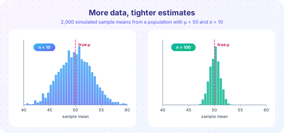
How do we decide whether an estimator is good? Imagine repeating the sampling many times and looking at the cloud of estimates, as in the picture.
Bias
The bias of an estimator θ̂ for a parameter θ is E[θ̂] − θ: how far the center of the cloud sits from the truth. An estimator is unbiased if its sampling distribution is centered on the parameter. The sample mean is unbiased, because by linearity of expectation
E[X̄] = (E[X1] + ... + E[Xn]) / n = (n · μ) / n = μ
Bias is about being right on average. An unbiased estimator can still be far off in any particular sample.
Variance and the standard error
The second feature is how widely the cloud spreads. If the observations are independent with variance σ², then
Var(X̄) = σ² / n so the standard deviation is σ / √n
The standard deviation of an estimator's sampling distribution is its standard error. With σ = 10 and n = 25, the standard error of the mean is 10 / 5 = 2. With n = 100 it is 10 / 10 = 1. Four times the data halves the typical error. The square root is the reason: to make estimates ten times as precise you need a hundred times as much data, which is why bigger samples have diminishing returns.
Mean squared error
Often we compare estimators by mean squared error, MSE = Bias² + Variance. A slightly biased estimator with much smaller variance can have a lower MSE than an unbiased but jumpy one. That trade-off between bias and variance returns later when we compare models.
Consistency
An estimator is consistent if it converges to the true parameter as the sample grows without limit. The law of large numbers says the sample mean is consistent: as n increases, X̄ gets arbitrarily close to μ. Consistency is weaker than unbiasedness. An estimator can be biased in small samples but consistent, and an unbiased estimator can be inconsistent (for instance, "use only the first observation" is unbiased but never improves with more data).
Econometricians often accept a small bias for consistency, but they treat a lack of consistency as fatal: an estimator that does not converge to the truth, even with infinite data, is simply wrong, and no amount of data will repair it. Chapter 6 explains one important way that happens.
The shape of the sampling distribution
For inference we want the shape of the cloud, not only its center and spread. The central limit theorem (CLT) delivers it: for independent observations with finite variance, the sample mean's sampling distribution becomes approximately normal as n grows, no matter how skewed the underlying data are:
(X̄ − μ) / (σ / √n) → Normal(0, 1)
Wages are right-skewed, yet the average wage of 100 workers behaves almost like a normal variable. This is why normal tables appear everywhere in testing. How large must n be? It depends on how skewed the data are; for mild skew, 30 is often enough, for extreme skew you may need hundreds.
Worked example: a bias that disappears
A common beginner estimator of the variance is (1/n) Σ (Xi − X̄)². It looks natural, yet it is biased: its expectation is ((n − 1)/n) σ². With n = 5 it hits only 80% of the truth on average. The reason is that X̄ is fitted to the same data, so the data sit closer to X̄ than to the true μ. Dividing by n − 1 instead, giving the sample variance s², exactly removes the bias. As n grows the factor (n − 1)/n tends to 1, so the biased version is still consistent.
The population, the sample and the estimate in practice
In applied work you have one sample, so you cannot draw the picture of the sampling distribution directly. You estimate its spread from the data: the estimated standard error is s / √n, where s is the sample standard deviation. A rough 95% confidence interval for the mean is then X̄ ± 1.96 · s / √n in large samples. We develop this properly in Chapter 4; here it is enough to see that a standard error converts your single estimate into a statement about how much it is likely to be off.
The same ideas govern a regression slope. The slope b1 is an estimator with a sampling distribution, centered (under assumptions we list in Chapter 4) at the true slope and shrinking in spread as n grows and as the spread of x grows. The simulation tools you use here are exactly what you will use to understand OLS.
Common misconceptions
"A 95% confidence interval contains the true value with 95% probability." More precisely, 95% of intervals built this way (over repeated samples) cover the truth. For the one you computed, the truth is either inside or not; the 95% describes the procedure.
"Unbiased means accurate." Unbiased means right on average. A wildly variable unbiased estimator can be a poor guide in any single sample.
"The standard error is the standard deviation of my data." The standard deviation describes how spread out individual observations are; the standard error describes how spread out the estimate would be across samples. It is smaller by the factor √n.
"A large sample can fix any estimator." Only a consistent estimator improves with more data. A badly biased or inconsistent estimator can be estimated precisely and wrongly.
Try it
First example: simulate the sampling distribution of the sample mean for three sample sizes and compare the observed spread with the formula σ / √n. The population here is invented, with mean 50 and standard deviation 10.
Press Run (or Ctrl + Enter) to see the result here.
Program input · what you'd type while the program runs
Type the answers before you press Run, one per line. Each time the program reads a line (with input()), it gets the next line from this box.
Second example: the bias of the "divide by n" variance estimator. We draw many small samples (n = 5) and average each version.
Press Run (or Ctrl + Enter) to see the result here.
Program input · what you'd type while the program runs
Type the answers before you press Run, one per line. Each time the program reads a line (with input()), it gets the next line from this box.
Third example: the central limit theorem in action. The population is strongly skewed (an exponential distribution, a rough stand-in for incomes), but the distribution of sample means becomes bell-shaped as n grows.
Press Run (or Ctrl + Enter) to see the result here.
Program input · what you'd type while the program runs
Type the answers before you press Run, one per line. Each time the program reads a line (with input()), it gets the next line from this box.
Check your understanding
Quick check · 5 questions
of 5 answered You scored / 5 · perfect!
-
1. Which of these is a fixed (non-random) quantity?
Parameters are fixed unknown numbers; estimators are random before sampling and estimates are fixed numbers after. -
2. If σ = 12 and n = 36, what is the standard error of the sample mean?
σ divided by √n is 12 / 6 = 2. -
3. An estimator that is biased in small samples but converges to the truth as n grows is
Consistency is convergence to the truth with growing n; it allows small-sample bias. -
4. The central limit theorem says that, for large n, the sampling distribution of the sample mean is approximately
Regardless of the population's shape (with finite variance), averages tend toward a normal distribution. -
5. What does a standard error tell you?
It is the standard deviation of the estimator's sampling distribution.
Summary
- Parameters are fixed; estimators are random rules; estimates are the numbers one sample produces.
- Judge estimators by bias, variance (standard error), mean squared error and consistency.
Var(X̄) = σ²/n: the standard error isσ/√n, so quadrupling the data halves it.- The law of large numbers gives consistency of the sample mean; the central limit theorem gives approximate normality.
- Dividing by
n − 1removes the bias of the sample variance.
Next: Chapter 2 review
Track your progress
Create a free account to tick off lessons and pick up where you left off on any device.
of Econometrics lessons completed