


















Lesson 14 of 49 · Simple and Multiple Regression
Multiple regression
Learn multiple linear regression: the model, how to interpret coefficients holding other variables fixed, the partialling-out idea, matrix OLS, adjusted R-squared and why simple and multiple slopes differ.
Wages depend on schooling, but also on experience, on the region, on the industry. If you regress wage on schooling alone, the slope mixes the effect of schooling with the effects of everything correlated with schooling. Multiple regression puts several explanatory variables in the equation at once, so that the coefficient on each one answers a sharper question: how does the outcome differ across people who are alike in all the other included variables?
That phrase, "holding other things constant" or the Latin ceteris paribus, is the reason multiple regression dominates empirical economics. This lesson explains how the model works, what exactly the software does to hold things constant, why simple and multiple slopes usually disagree, and how to read the output.
What you will learn
- The multiple regression model and how to interpret its coefficients.
- The partialling-out (Frisch-Waugh-Lovell) result behind "holding other things constant".
- Why the coefficient on
x1changes when you addx2. - How adjusted R-squared works and what perfect collinearity means.
Key terms
Multiple regression: a regression with two or more explanatory variables.
Ceteris paribus: "other things equal", the comparison a coefficient describes.
Partial effect: the change in the expected outcome per one-unit change in one regressor, others fixed.
Adjusted R-squared: R-squared with a penalty for the number of regressors.
Perfect collinearity: an exact linear relationship among regressors that makes coefficients impossible to separate.
The model
With k explanatory variables, the population model is
y = β0 + β1·x1 + β2·x2 + ... + βk·xk + u
and the OLS fitted equation is ŷ = b0 + b1·x1 + ... + bk·xk. OLS still minimizes the sum of squared residuals. With two regressors the "line" becomes a plane; with more, a hyperplane that you cannot draw, though the algebra is the same.
Interpretation
A fitted equation such as
wage-hat = −3.0 + 0.90·educ + 0.25·exper
(an invented example, wage in dollars per hour, educ and exper in years) is read coefficient by coefficient:
0.90oneduc: comparing two workers with the same experience, the one with one more year of schooling earns on average $0.90 more per hour.0.25onexper: comparing two workers with the same schooling, one more year of experience goes with $0.25 more per hour.- The prediction for a worker with 16 years of schooling and 10 years of experience is
−3.0 + 0.90 × 16 + 0.25 × 10 = −3.0 + 14.4 + 2.5 = 13.9dollars per hour.
Each coefficient is a partial effect in the descriptive sense: the difference across people matched on the other variables. It is still not automatically causal; unincluded factors may remain in u.
What "holding other things constant" means in practice
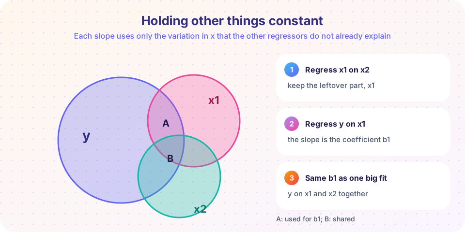
The software does not hunt for workers with identical experience. It uses algebra that has the same effect, called partialling out (the Frisch-Waugh-Lovell theorem). To get the coefficient on x1 in a regression with x2:
- Regress
x1onx2and keep the residualsx̃1. These are the part ofx1thatx2cannot predict. - Regress
yonx̃1(a simple regression). The slope is exactlyb1from the full regression.
In the Venn picture, x1 and x2 overlap: some of the variation in schooling is shared with experience. The coefficient on x1 is computed only from the part of x1 outside the overlap with x2 (the region A in the picture), and that part's relation with y. The shared region B is credited to neither, which is why variables that are strongly related to each other produce imprecise coefficients (Chapter 4).
You can also stress the logic from the other side: the coefficient on x1 is identified only from variation in x1 that is independent of the other included variables. If x1 is almost entirely predicted by the others, little independent variation remains, and the estimate is unstable.
Why simple and multiple slopes differ
The slope from regressing y on x1 alone, call it b̃1, and the multiple-regression slope b1 are linked by an exact sample identity when there are two regressors:
b̃1 = b1 + b2 · δ1
where b2 is the coefficient on x2 in the multiple regression and δ1 is the slope from regressing x2 on x1. In words: the simple slope picks up the direct effect of x1 (b1) plus the effect that runs through x2 (how x2 changes with x1, times how much x2 matters).
The two slopes coincide in only two cases: when b2 = 0 (the omitted variable does not matter) or when δ1 = 0 (it is uncorrelated with x1). This identity is the algebra behind omitted variable bias in Chapter 4.
Worked example
Suppose in a sample, experience declines as schooling rises: regressing exper on educ gives slope δ1 = −1.0 (more schooling means fewer years in the labor market at a given age). The multiple regression has b1 = 1.0 for schooling and b2 = 0.3 for experience. Then the simple-regression slope is
b̃1 = 1.0 + 0.3 × (−1.0) = 0.7
Ignoring experience, the estimated return to a year of schooling is understated, because more schooled workers have less experience and experience pays. The simulation below reproduces this.
Matrix form, briefly
With many regressors we write the model for all observations in one line. Let y be the n × 1 vector of outcomes and X the n × (k + 1) matrix whose first column is all ones (for the intercept) and whose other columns hold the regressors. The OLS solution is
b = (X′X)⁻¹ X′y
This is the same set of normal equations as before, solved in one step. The formula requires that X′X can be inverted, which happens exactly when no column of X is an exact linear combination of the others. If one is (say, you include both a "male" and a "female" dummy together with an intercept), the software cannot separate their effects. This perfect collinearity makes coefficients impossible to compute: that is the dummy variable trap, handled in the next lesson. In practice software drops a variable or reports an error.
Adjusted R-squared
Adding a regressor can only raise the plain R², even when it is pure noise. The adjusted R-squared corrects for this:
adj R² = 1 − (1 − R²) · (n − 1) / (n − k − 1)
The factor (n − 1)/(n − k − 1) grows with k, so adding a variable raises adjusted R-squared only if the improvement in fit outweighs the penalty. With R² = 0.40, n = 50 and k = 3 we get 1 − 0.60 × 49/46 ≈ 0.361. Adjusted R-squared can fall, and can be negative. It is a rough guide to model comparison, not a substitute for thinking.
Common misconceptions
"Controlling for a variable removes its influence entirely." Controls remove the linear association with the included variable. If the true relation is nonlinear, or if you measured the control with error, some influence remains.
"More controls always make an estimate more credible." Adding the wrong variables, such as ones that are themselves consequences of the variable of interest, can create bias. Control for confounders, not for mediators or consequences.
"A coefficient is the effect, whatever else is in the model." A coefficient's meaning and size depend on which other variables are included. Always say "holding X, Y and Z constant".
Try it
First example: simulate wages from a known rule, compute OLS with the matrix formula and compare with the true parameters. The data are invented; the true coefficients are 2, 1.0, 0.3.
Press Run (or Ctrl + Enter) to see the result here.
Program input · what you'd type while the program runs
Type the answers before you press Run, one per line. Each time the program reads a line (with input()), it gets the next line from this box.
Second example: verify the partialling-out result and the identity linking the simple and multiple slopes, on the same data.
Press Run (or Ctrl + Enter) to see the result here.
Program input · what you'd type while the program runs
Type the answers before you press Run, one per line. Each time the program reads a line (with input()), it gets the next line from this box.
Third example: why raw R-squared is a poor guide. We add 0 to 30 columns of pure noise to a regression and track R² and adjusted R².
Press Run (or Ctrl + Enter) to see the result here.
Program input · what you'd type while the program runs
Type the answers before you press Run, one per line. Each time the program reads a line (with input()), it gets the next line from this box.
Check your understanding
Quick check · 5 questions
of 5 answered You scored / 5 · perfect!
-
1. In wage-hat = −3.0 + 0.90·educ + 0.25·exper, the 0.25 means
A coefficient in multiple regression compares workers who are alike in the other included variables. -
2. What does partialling out do to get the coefficient on x1?
The coefficient comes from the residual of x1 after regressing it on the other regressors. -
3. With b1 = 1.0, b2 = 0.3 and δ1 = −1.0, the simple-regression slope of y on x1 is
b̃1 = b1 + b2·δ1 = 1.0 + 0.3(−1.0) = 0.7. -
4. Including both a 'male' and a 'female' dummy together with an intercept causes
male + female = 1 equals the intercept column, so the coefficients cannot be separated. -
5. Adjusted R-squared differs from R-squared because it
It multiplies the unexplained share by (n − 1)/(n − k − 1), a penalty that grows with k.
Summary
- Multiple regression adds regressors; each coefficient compares units that are alike in the other included variables.
- OLS solves
b = (X′X)⁻¹X′y; the coefficient onx1uses only the part ofx1not explained by the other regressors. - The simple and multiple slopes are linked by
b̃1 = b1 + b2·δ1, so they differ when the omitted variable matters and is correlated withx1. - Perfect collinearity makes coefficients impossible to separate.
- Plain R-squared never falls with extra regressors; adjusted R-squared penalizes them.
Track your progress
Create a free account to tick off lessons and pick up where you left off on any device.
of Econometrics lessons completed