


















Lesson 7 of 49 · Data and the Regression Idea
Probability and expectation review
Review the probability tools behind regression: random variables, expectation, variance, covariance, correlation and the normal distribution, with worked examples and simulations.
Econometrics treats data as the outcome of a chance process. A person's wage is partly explained by schooling and experience and partly by things that look like luck. To reason about such quantities we need a small vocabulary: random variable, distribution, expectation, variance, covariance. You may have met these in a statistics course; this lesson refreshes exactly the parts regression uses, with an eye on the questions you will face later.
If any of this feels rusty, do not worry. The lesson is written so you can read it from scratch.
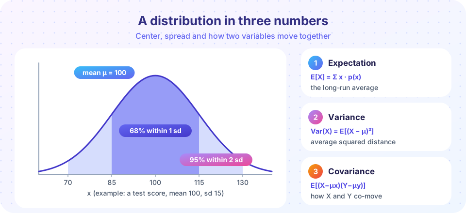
What you will learn
- What a random variable and its distribution are.
- How to compute an expectation, a variance and a standard deviation by hand.
- The rules of expectation and variance you will use constantly.
- What covariance and correlation measure, and how the normal distribution behaves.
Key terms
Random variable (X): a numerical outcome of a chance process. Capital letters denote the variable; lowercase letters denote particular values.
Probability distribution: the list (or curve) of how likely each value is.
Expected value, E[X]: the probability-weighted average of the possible values.
Variance, Var(X): the expected squared deviation from the mean.
Covariance, Cov(X, Y): the expected product of deviations from the means.
Random variables and distributions
A random variable assigns a number to each possible outcome of a chance process. Roll a die: the face value is a random variable. Choose a worker at random from a country: that worker's wage is a random variable. It is discrete if it takes separate values (die faces, number of children) and continuous if it can take any value in a range (wages, heights).
For a discrete variable the distribution is a list of probabilities p(x) that add up to 1. For a continuous variable it is a density curve, where the area under the curve between two values is the probability of landing in that range. A single exact value has probability zero; only intervals have probability.
Expectation
The expected value or mean of a discrete random variable is
E[X] = Σ x · p(x)
It is not necessarily a value the variable can take, and it is not a prediction of one trial; it is the long-run average. Roll a fair die thousands of times and the average approaches 3.5, even though 3.5 is not a face.
Worked example: a loaded die
Suppose a loaded die lands on 1, 2, 3, 4 with probability 0.1 each, on 5 with probability 0.2 and on 6 with probability 0.4. These add to 1.
E[X] = 0.1(1) + 0.1(2) + 0.1(3) + 0.1(4) + 0.2(5) + 0.4(6)
     = 1.0 + 1.0 + 2.4 = 4.4
The expected face is 4.4, noticeably above the fair die's 3.5 because the die favors large numbers.
Rules of expectation
These three rules are used on nearly every page of the course.
- Constants:
E[c] = c. - Linearity:
E[aX + b] = a·E[X] + b. - Sums:
E[X + Y] = E[X] + E[Y], always, whether or not X and Y are independent.
Linearity is surprisingly powerful. If the wage rule is wage = 3 + 1.1·educ + u and the average schooling is 13 years with E[u] = 0, the average wage is 3 + 1.1 × 13 + 0 = 17.3 dollars. You did not need the distribution of anything, only the mean.
Variance and standard deviation
The variance measures spread:
Var(X) = E[(X − μ)²] = E[X²] − μ² where μ = E[X]
The standard deviation σ = √Var(X) is in the same units as X, which makes it easier to read. Continuing the loaded die, first E[X²] = 0.1(1 + 4 + 9 + 16) + 0.2(25) + 0.4(36) = 3 + 5 + 14.4 = 22.4. Then Var(X) = 22.4 − 4.4² = 22.4 − 19.36 = 3.04, so σ ≈ 1.74.
Rules of variance
Var(aX + b) = a²·Var(X): shifting does not change spread, and scaling byascales spread by|a|(variance bya²).Var(X + Y) = Var(X) + Var(Y) + 2·Cov(X, Y).- If
XandYare independent,Cov(X, Y) = 0, so variances simply add.
A frequent slip is to write Var(X + Y) = Var(X) + Var(Y) without the covariance term. It is correct only if the two are uncorrelated.
Covariance and correlation
Covariance measures whether two variables tend to move together:
Cov(X, Y) = E[(X − μX)(Y − μY)]
When X is above its mean, is Y usually above its mean too? If so, products of deviations are mostly positive and the covariance is positive. If one tends to be high when the other is low, it is negative. Zero covariance means no linear tendency.
The trouble with covariance is its units: dollars times years. The correlation removes them:
Corr(X, Y) = Cov(X, Y) / (σX · σY) always between −1 and 1
Worked example with a small sample
Take three pairs (x, y): (1, 2), (2, 4), (3, 9). The means are x̄ = 2 and ȳ = 5. The deviations for x are −1, 0, 1 and for y are −3, −1, 4. The products are 3, 0, 4, which sum to 7. The sample covariance is 7 / (3 − 1) = 3.5. The sample variances are (1 + 0 + 1)/2 = 1 for x and (9 + 1 + 16)/2 = 13 for y, so the correlation is 3.5 / (1 × √13) ≈ 0.97, a strong positive relationship.
Covariance will reappear immediately: the slope of the least squares line is exactly Cov(x, y) / Var(x). In the example, 3.5 / 1 = 3.5, which is the slope of the line of best fit through those three points.
The normal distribution
The normal (bell-shaped) distribution appears everywhere because of the central limit theorem, which we meet in Lesson 3. It is completely described by its mean μ and standard deviation σ. For any normal variable:
- about 68% of values lie within one standard deviation of the mean,
- about 95% lie within two (more exactly 1.96),
- about 99.7% lie within three.
A standard normal variable has μ = 0 and σ = 1. Any normal X can be standardized: Z = (X − μ) / σ is standard normal. For a score distribution with mean 100 and standard deviation 15, a value of 130 has Z = (130 − 100) / 15 = 2, which is two standard deviations above the mean, and only about 2.3% of people exceed it. Standardizing lets one table (or one function) cover all normal distributions.
Common misconceptions
"The expected value is the most likely value." It is the average, which may be impossible (3.5 on a die) or rare. The most likely value is the mode.
"Uncorrelated means independent." Independence implies zero correlation, but not the other way round. If X is symmetric around 0 and Y = X², then Y depends entirely on X, yet their correlation is zero.
"Variance adds up always." Only when variables are uncorrelated. Otherwise the covariance term matters, and a negative covariance can make a sum less variable than its parts (this is the logic of diversification in finance).
Try it
The first example computes the loaded die's expectation and variance exactly and then checks them by simulation. Close agreement between the formula and the simulation is how statisticians gain confidence that they understood the concept.
Press Run (or Ctrl + Enter) to see the result here.
Program input · what you'd type while the program runs
Type the answers before you press Run, one per line. Each time the program reads a line (with input()), it gets the next line from this box.
The second example shows how correlation changes as the relationship gets noisier, and how covariance relates to the slope. The pink line is the least squares fit, whose slope is Cov(x, y) / Var(x).
Press Run (or Ctrl + Enter) to see the result here.
Program input · what you'd type while the program runs
Type the answers before you press Run, one per line. Each time the program reads a line (with input()), it gets the next line from this box.
The third example shows the 68-95-99.7 rule empirically for the score distribution used in the picture above.
Press Run (or Ctrl + Enter) to see the result here.
Program input · what you'd type while the program runs
Type the answers before you press Run, one per line. Each time the program reads a line (with input()), it gets the next line from this box.
Check your understanding
Quick check · 5 questions
of 5 answered You scored / 5 · perfect!
-
1. A fair six-sided die has an expected value of
The average of 1 through 6 is 21/6 = 3.5. -
2. If E[X] = 10, what is E[3X + 2]?
By linearity, E[3X + 2] = 3·10 + 2 = 32. -
3. If Var(X) = 4, what is Var(3X + 2)?
Adding 2 does not change variance, and multiplying by 3 multiplies variance by 9, so 9 · 4 = 36. -
4. What does a covariance of zero tell you?
Zero covariance rules out a linear association but not a nonlinear dependence. -
5. For a normal variable with mean 100 and standard deviation 15, about what share lies between 70 and 130?
70 and 130 are two standard deviations from the mean, which contain about 95%.
Summary
- A random variable's distribution is summarized by its expectation (center) and variance (spread).
- Expectation is linear:
E[aX + b] = aE[X] + bandE[X + Y] = E[X] + E[Y]. Var(aX + b) = a²Var(X)andVar(X + Y) = Var(X) + Var(Y) + 2Cov(X, Y).- Covariance measures linear co-movement; correlation rescales it to between −1 and 1.
- The normal distribution has the 68-95-99.7 rule and can be standardized with
Z = (X − μ)/σ.
Track your progress
Create a free account to tick off lessons and pick up where you left off on any device.
of Econometrics lessons completed