


















Lesson 23 of 49 · Violations: Heteroskedasticity and Autocorrelation
Chapter 5 overview: when the error assumptions break
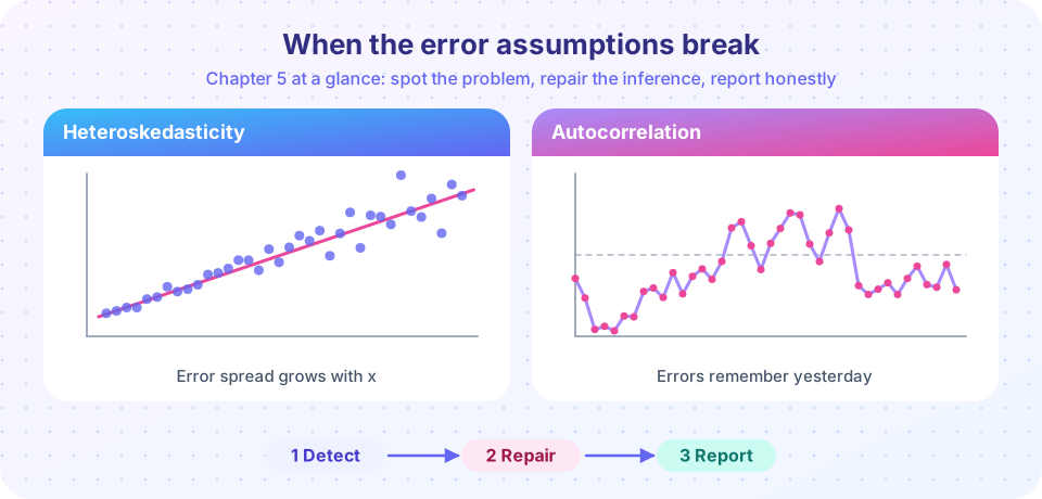
A map of chapter 5: why uneven error variance and serial correlation break standard errors, and how to detect, repair and report them.
Ordinary least squares is forgiving about many things, but not about everything. In the earlier chapters you met the classical assumptions: the model is linear in its parameters, the regressors are not perfectly collinear, the errors have mean zero given the regressors, and the errors have constant variance and are uncorrelated with each other. When the first three hold, OLS gives unbiased coefficients. When the last two fail, the coefficients are still unbiased, but the standard errors you print in your results table are wrong. Your t statistics, p-values and confidence intervals then tell a story the data do not support.
This chapter is about those last two assumptions. Breaking the first is called heteroskedasticity: the spread of the errors depends on the regressors. Breaking the second is called autocorrelation (or serial correlation): the error today is related to the error yesterday. Both are routine in real data. Household spending varies far more among rich households than among poor ones. Quarterly inflation does not reset every three months; it carries momentum.
What you will learn
- Why OLS stays unbiased but its standard errors go wrong when variance is uneven or errors are correlated.
- How to look for the problem with plots first and formal tests second.
- How to repair inference with robust (HC and HAC) standard errors, and when weighted least squares is better.
- How to describe what you found and what you did in a way a reader can check.
Key terms
Heteroskedasticity: the variance of the error term changes with the regressors. Homoskedasticity: the variance is constant. Autocorrelation: the errors in different observations, usually neighbouring time periods, are correlated. Robust standard errors: standard errors that stay valid when the variance is uneven. HAC: heteroskedasticity and autocorrelation consistent standard errors, used for time series.
The big picture in five slides
What OLS promises
What breaks
What it costs
How to find it
How to fix it
Why the standard error is the thing that breaks
Recall the sampling variance of the slope in a simple regression under the classical assumptions: Var(b1) = σ² / Σ(xi − x̄)². This formula takes one common σ² for every observation. If the real error variance differs from one observation to the next, the true variance of b1 is a weighted sum with different weights, and the textbook formula is simply the wrong calculation. It can be too small, which makes you over-confident, or too large, which hides real effects. There is no general rule about the direction, though the most common case in economics, with variance growing in the regressor, tends to make the usual standard errors too small.
The same logic holds for autocorrelation. If the errors of neighbouring quarters are positively correlated, each new observation carries less new information than the formula assumes. You have, in effect, fewer independent data points than your sample size says. The usual standard errors are then typically too small, sometimes dramatically so.
A good habit follows from this. Never treat a regression table as finished until you have asked: are these standard errors believable for this kind of data? For cross-sectional data the main worry is heteroskedasticity. For time series the worry is autocorrelation, and often both.
A quick demonstration
Below, we simulate a world where the true slope is exactly zero, but the error spread grows with x. We then ask how often the usual t test falsely declares the slope "significant" at the 5% level. If the usual standard errors were right, the answer would be about 5%.
Press Run (or Ctrl + Enter) to see the result here.
Program input · what you'd type while the program runs
Type the answers before you press Run, one per line. Each time the program reads a line (with input()), it gets the next line from this box.
This is a labelled simulation, not real data. Run it a few times with different seeds and watch how the usual rejection rate stays above the nominal 5% while the robust version sits closer to it. By the end of the chapter you will be able to explain both numbers.
What each lesson covers
- What heteroskedasticity is: the definition, where it comes from in real data, and exactly what it breaks.
- Testing for heteroskedasticity: residual plots, the Breusch-Pagan and White tests, and what a rejection does and does not tell you.
- Robust errors and weighted least squares: the HC family, when to prefer WLS, and the feasible GLS idea.
- Serial correlation: AR(1) errors, the Durbin-Watson and Breusch-Godfrey tests, and Newey-West standard errors.
- Chapter review: one picture, a recap table and a long quiz.
Common misconceptions
"Heteroskedasticity biases my coefficients." It does not. Under the other assumptions, OLS slopes stay unbiased and consistent. What fails is the standard error, and with it the t test, the F test and the confidence interval.
"Autocorrelation only matters for fancy time-series models." It matters for any regression on ordered data, including a plain trend regression, and it can also appear in cross-sectional data with geographic or group structure.
Check your understanding
Quick check · 4 questions
of 4 answered You scored / 4 · perfect!
-
1. Under heteroskedasticity, which OLS output is the main thing that becomes unreliable?
The slopes stay unbiased; the formula for their variance assumed a single common error variance and no longer matches the data. -
2. Positive autocorrelation in the errors usually makes the usual OLS standard errors...
Positively correlated errors carry less independent information than the sample size suggests, so the standard errors are typically too small. -
3. Which pair of terms is matched correctly?
Autocorrelation is correlation among the errors themselves; correlation between errors and regressors is endogeneity, which is chapter 6. -
4. In the simulation above, the true slope is zero. What does a false-alarm rate far above 5% tell you?
A correct 5% test should reject a true null about 5% of the time. A higher rate means the usual standard errors are too small.
Summary
- Heteroskedasticity and autocorrelation leave OLS slopes unbiased but break the usual standard errors.
- The workflow is detect, repair, report: plots first, tests second, robust or modelled errors third.
- Cross-sections suggest heteroskedasticity; time series suggest autocorrelation, often together.
- Robust standard errors repair inference; WLS and GLS can also improve efficiency when the structure is known.
Track your progress
Create a free account to tick off lessons and pick up where you left off on any device.
of Econometrics lessons completed