


















Lesson 36 of 49 · Panel Data and Time Series
Stationarity and unit roots
Learn what stationarity means, how a random walk differs from a stationary AR(1), and how to run and read the augmented Dickey-Fuller test in Python.
A time series regression has a hidden assumption that cross-section regressions do not need to spell out: the future must resemble the past in a statistical sense. If the average, the spread and the dependence structure of a series keep changing, then a relationship estimated on one stretch of the data tells you little about another, and the usual t and F tests lose their meaning.
Stationarity is the formal version of "the future resembles the past". This lesson defines it, contrasts the stationary AR(1) process with the random walk, explains the difference between a trend and a unit root, and teaches the Dickey-Fuller test that economists use to tell them apart.
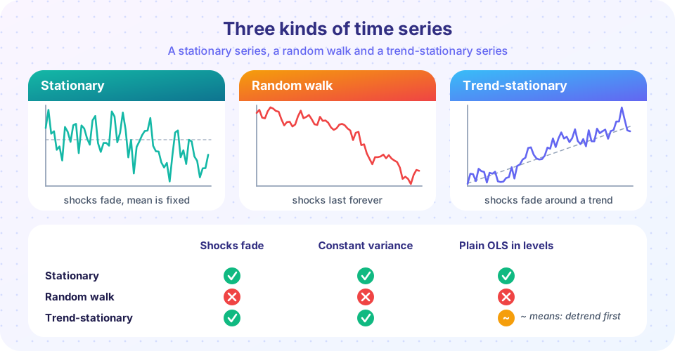
What you will learn
- The definition of weak stationarity and why it matters for inference.
- How the AR(1) coefficient
φseparates stationary series from random walks. - The difference between trend-stationary and difference-stationary series.
- How to run the (augmented) Dickey-Fuller test, read its critical values and difference a series when needed.
Key terms
Weak stationarity: constant mean, constant finite variance, and autocovariances that depend only on the lag. White noise: uncorrelated shocks with mean zero and constant variance. Random walk: yt = yt−1 + εt. Integrated of order d, I(d): a series that becomes stationary after differencing d times. ADF test: augmented Dickey-Fuller test of the null hypothesis that a series has a unit root.
Weak stationarity
A series yt is weakly stationary if three conditions hold for all t:
E(yt) = μdoes not depend ont.Var(yt) = σ²is finite and does not depend ont.Cov(yt, yt−h) = γ(h)depends only on the lagh, not ont.
Think of a thermometer reading in a room with a thermostat: it wanders but keeps returning to the set temperature, and the wandering looks the same in January as in July. By contrast, the price level of a country over fifty years has no fixed mean to return to.
The AR(1) process: stationary or not?
The simplest model with memory is the first-order autoregression
yt = φ yt−1 + εt, εt white noise
with three regimes.
|φ| < 1: stationary. A shockεtoday has an effectφʰafterhperiods, which decays geometrically. The mean is zero, the variance isσ²/(1 − φ²), and the autocorrelation at laghisφʰ.φ = 1: random walk,yt = yt−1 + εt = y0 + ε1 + ... + εt. The shocks accumulate, the variance ist σ²and grows without bound, and the series has no mean to revert to. We say the process has a unit root.|φ| > 1: explosive; rare in economics.
Adding a constant gives a random walk with drift: yt = δ + yt−1 + εt, which wanders around an upward (or downward) sloping path. The first difference Δyt = yt − yt−1 of a random walk is stationary (white noise plus the drift), so a random walk is integrated of order one, I(1). A stationary series is I(0).
Trend or unit root?
Many macro series trend upward. Two very different stories produce a trend.
- Trend-stationary:
yt = a + bt + utwithutstationary. The series fluctuates around a deterministic line; shocks fade. The correct treatment is to subtract the trend (regress ont). - Difference-stationary:
yt = δ + yt−1 + εt. Shocks are permanent. The correct treatment is to difference the series.
The distinction is practical and philosophical: does a recession leave a permanent mark on output, or does the economy bounce back to its trend? Nelson and Plosser (1982) famously argued that most US macroeconomic series look like unit-root processes. Applying the wrong cure is costly: detrending a random walk does not make it stationary, and differencing a trend-stationary series introduces unnecessary noise (over-differencing).
The Dickey-Fuller test
Subtract yt−1 from both sides of the AR(1): Δyt = (φ − 1) yt−1 + εt = γ yt−1 + εt, with γ = φ − 1. The unit root hypothesis is
H0: γ = 0 (unit root) versus H1: γ < 0 (stationary)
Dickey and Fuller (1979) showed that the usual t statistic on γ̂ does not follow a t distribution under H0. It follows a different distribution, shifted to the left, so we need special critical values. The test comes in three flavours, according to the deterministic terms in the regression:
| Regression | Use when | 1% | 5% | 10% |
|---|---|---|---|---|
| No constant | series fluctuates around zero | −2.58 | −1.95 | −1.62 |
| Constant | series fluctuates around a nonzero mean | −3.43 | −2.86 | −2.57 |
| Constant and trend | series may trend | −3.96 | −3.41 | −3.12 |
(Asymptotic MacKinnon values; they change slightly with sample size.) Reject the unit root when the t statistic is more negative than the critical value.
The augmented Dickey-Fuller (ADF) test adds lagged differences to soak up serial correlation in the error:
Δyt = α + δt + γ yt−1 + Σj=1..p ψj Δyt−j + εt
Choose p by an information criterion (AIC, BIC) or by testing that the residuals are white noise. The critical values are the same as above.
Some cautions:
- Low power. The test has trouble telling a unit root from a root like 0.98, especially in short samples.
- Deterministic terms matter. If you include a trend when there is none you lose power; if you leave out a trend that is there, you may fail to reject falsely.
- Opposite null. The KPSS test has stationarity as the null. Using both tests gives a more complete picture: ADF rejects and KPSS does not reject means stationary; the reverse means unit root; mixed results mean the data are uninformative.
- Structural breaks mimic unit roots: a one-off shift in the mean makes tests fail to reject.
ADF by hand
The function below implements the ADF regression with a constant, using the t statistic on yt−1. We apply it to a stationary AR(0.6), a random walk and a trend-stationary series, all simulated.
Press Run (or Ctrl + Enter) to see the result here.
Program input · what you'd type while the program runs
Type the answers before you press Run, one per line. Each time the program reads a line (with input()), it gets the next line from this box.
The stationary series should reject the unit root clearly (a very negative t). The random walk should not reject (a true unit root is still rejected in about 5% of samples, so with an unlucky seed you may see an exception). The trend-stationary series is the instructive case: with only a constant, the unit-root test often fails to reject; with a trend term it rejects. Differencing the random walk produces a series that rejects.
The shifted distribution
Why do we need special critical values? Simulate the Dickey-Fuller t statistic under the null of a unit root and compare it with a standard normal distribution.
Press Run (or Ctrl + Enter) to see the result here.
Program input · what you'd type while the program runs
Type the answers before you press Run, one per line. Each time the program reads a line (with input()), it gets the next line from this box.
The simulated distribution is skewed and shifted to the left of the normal. Its 5% point is close to −2.86, which is why the table says so.
What to do after the test
- Unit root rejected (series is stationary): use it in levels.
- Unit root not rejected: difference the series. Check that the differences are stationary, and interpret the coefficients as relationships among changes (growth rates if you took log differences).
- Several nonstationary series that you want in levels: test for cointegration (next lesson) before differencing away potentially valuable long-run information.
- Remember that tests can be wrong; plot the series, look at its autocorrelation function and think about whether economic theory says shocks should be permanent.
Common misconceptions
"If the ADF test fails to reject, the series definitely has a unit root." Failing to reject reflects low power as much as truth, especially for near-unit-root persistence.
"A trending series must have a unit root." It might be trend-stationary. The test must include the right deterministic terms.
"Differencing is always safe." Differencing a stationary series creates a non-invertible moving-average error and throws away long-run information.
"A stationary series cannot trend." A deterministic trend is allowed under trend-stationarity; it is the stochastic trend that signals a unit root.
Check your understanding
Quick check · 5 questions
of 5 answered You scored / 5 · perfect!
-
1. In yt = phi y(t-1) + e(t), which value of phi gives a random walk?
phi = 1 means shocks accumulate and the series has a unit root. -
2. A series is I(1). After taking first differences it is...
I(1) means one difference makes the series stationary. -
3. The null hypothesis of the Dickey-Fuller test is...
The test starts from a unit root and looks for evidence of stationarity. -
4. A Dickey-Fuller t statistic is -2.1 with a constant (5% critical value -2.86). Conclusion?
-2.1 is not more negative than -2.86, so we cannot reject a unit root at 5%. -
5. Which statement about KPSS is correct?
KPSS reverses the null, which is why the two are used together.
Summary
- Weak stationarity requires a constant mean, constant variance and autocovariances that depend only on the lag.
- In an AR(1),
|φ| < 1is stationary andφ = 1is a random walk whose shocks never fade; random walks are I(1). - Trend-stationary series are detrended; difference-stationary series are differenced.
- The ADF test has a unit root as its null and uses non-standard critical values (for example −2.86 at 5% with a constant); it has low power.
Track your progress
Create a free account to tick off lessons and pick up where you left off on any device.
of Econometrics lessons completed