


















Lesson 39 of 49 · Causal Methods and Practice
Chapter 8 overview: a ladder of causal designs
A map of chapter 8: potential outcomes, randomized trials, difference-in-differences and regression discontinuity, and how design choices drive credibility.
Most of the questions that make people interested in economics are causal. Did the minimum wage reduce employment? Did a training program raise earnings? Does a tax credit change how much people work? A regression coefficient is only a number, but it is always offered as an answer to such a question. Whether it deserves that role is not a matter of software or sample size. It is a matter of design: how the data came to exist, and why the units that received the treatment can be compared with those that did not.
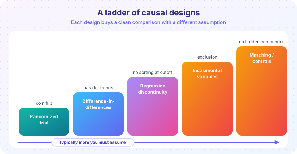
This chapter changes how you think about empirical work. Instead of starting with an estimator and hoping the assumptions hold, you will start with a clear causal question, write down what you would need to observe, and then pick a research design that makes the comparison credible. The designs form a kind of ladder: some need very little to be believed (a randomized experiment), others lean on stronger assumptions that you must argue for.
What you will learn
- The potential-outcomes framework and the fundamental problem of causal inference.
- Why randomization solves the problem, and what happens when it is not available.
- How difference-in-differences and regression discontinuity create comparisons from policy rules.
- How to judge a design by its identifying assumption rather than by its estimator.
Key terms
Treatment D: the intervention, coded 1 if received and 0 otherwise. Potential outcomes Y(1), Y(0): what the outcome would be with and without treatment. ATE: average treatment effect, E[Y(1) − Y(0)]. Selection bias: the difference between treated and untreated units even without treatment. Identification: the assumptions under which a causal effect can be recovered from data.
The chapter in five slides
The question
The obstacle
Experiments
Natural comparisons
Credibility
From regression to causation
In earlier chapters you estimated y = β0 + β1 x + u and learned conditions under which β̂1 is unbiased. The causal-inference tradition asks a prior question: what is the object we want to estimate, and could any dataset reveal it? Consider an education program. Person i has two potential outcomes: Yi(1), earnings if enrolled, and Yi(0), earnings if not. The causal effect for person i is Yi(1) − Yi(0), but we can never observe both. A simple comparison of enrolled and non-enrolled people's average earnings equals
E[Y | D = 1] − E[Y | D = 0] = E[Y(1) − Y(0) | D = 1] + { E[Y(0) | D = 1] − E[Y(0) | D = 0] }
The first term is the effect on the treated; the term in braces is selection bias: how much the treated would have earned even without treatment, compared with the non-treated. If more motivated people enroll, the bias is positive and the naive comparison overstates the effect. Every design in this chapter is a strategy for removing or bounding that second term.
A simulation of selection
In this invented example the true effect is exactly 2.0 for everybody. Motivated people enroll more often and would earn more without the program. A naive comparison is biased; a randomized assignment recovers the truth.
Press Run (or Ctrl + Enter) to see the result here.
Program input · what you'd type while the program runs
Type the answers before you press Run, one per line. Each time the program reads a line (with input()), it gets the next line from this box.
The self-selected comparison sits far above the truth because the treated group would have earned more anyway. The randomized comparison is centred on 2.0.
What each lesson covers
- Potential outcomes and randomized trials: the framework, ATE and related effects, why randomization works and what it cannot do.
- Difference-in-differences: comparing changes over time, the parallel-trends assumption and its checks.
- Regression discontinuity: treatment assigned by a threshold, local comparisons and bandwidth choices.
- Chapter review: the whole ladder in one picture and a ten-question quiz.
Common misconceptions
"Adding more controls makes a regression causal." Controls help only for confounders you can measure and only if you control for the right ones. Design, not a long list of covariates, creates credibility.
"Causal inference needs an experiment." Experiments are the cleanest route; the other designs substitute assumptions that you must defend with evidence.
Check your understanding
Quick check · 4 questions
of 4 answered You scored / 4 · perfect!
-
1. What is the fundamental problem of causal inference?
Each unit reveals only one of Y(1) and Y(0), so the individual effect is never directly observed. -
2. Selection bias is the difference between treated and untreated units in...
It equals E[Y(0) | D=1] - E[Y(0) | D=0]. -
3. Why does randomization remove selection bias?
A coin flip makes the groups comparable in everything, observed or not, on average. -
4. A self-selected treatment where motivated people enroll biases the naive comparison...
Motivated people would earn more even without the program, so the comparison overstates the effect.
Summary
- Causal effects are contrasts between potential outcomes; only one of them is ever observed per unit.
- A naive comparison equals the effect on the treated plus selection bias.
- Randomization, difference-in-differences and regression discontinuity are different ways to remove or argue away that bias.
- Judge any estimate by its identifying assumption and the checks that support it.
Track your progress
Create a free account to tick off lessons and pick up where you left off on any device.
of Econometrics lessons completed