


















Lesson 49 of 49 · Projects and Practice
Further study: where to go from here
A roadmap beyond this course: modern causal inference, time-series models, panel methods, machine learning for prediction and the tools and tracks to learn next.
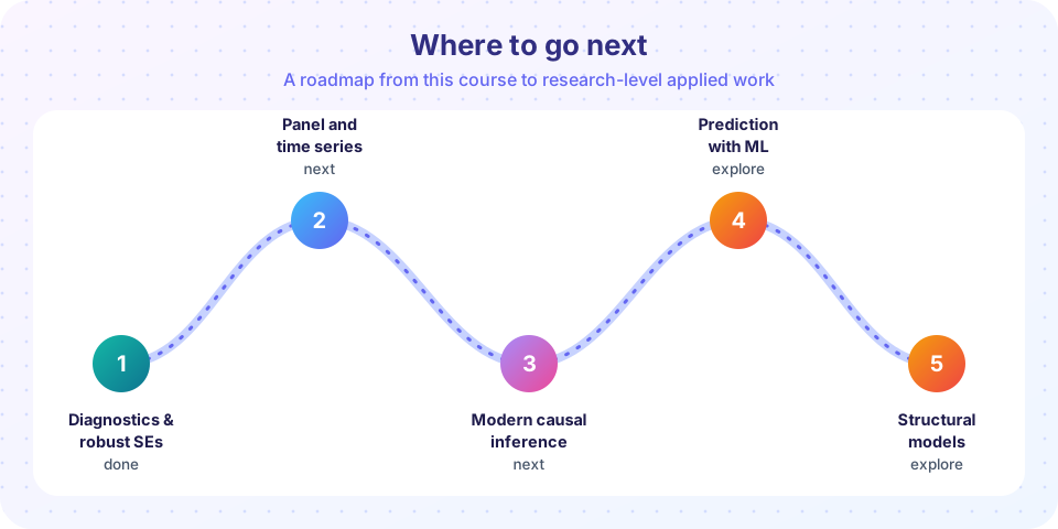
You have now seen the core of applied econometrics: regression and its assumptions, what happens when they break, instruments, panels, time series and the designs that turn an estimate into a causal claim. That is a solid foundation, and the honest next step is not "more of the same" but depth in the direction your work needs. This lesson sketches several directions, what each adds, and how to practise. Pick the one that matches the questions you want to answer, not the one that sounds most impressive.
What you will learn
- Five directions for further study and what each one adds.
- Which books and papers to read (as names to look for, not text to copy).
- How to connect this course to the other tracks on the site.
Key terms
Applied microeconometrics: estimating the effects of policies and choices on individuals and firms. Macroeconometrics: modelling aggregate time series. Structural estimation: estimating the parameters of an economic model rather than a reduced-form effect. Prediction versus causation: forecasting an outcome well is a different goal from learning what happens if you intervene. Replication: rerunning published analyses with their data.
Direction 1: deeper causal inference
The designs of chapter 8 have grown a large literature. Topics worth studying next:
- Modern difference-in-differences with staggered adoption: group-time effects, event-study estimators robust to heterogeneity (Callaway and Sant'Anna; Sun and Abraham; de Chaisemartin and D'Haultfœuille).
- Synthetic control: build a weighted combination of untreated units that matches the treated unit's pre-treatment path, ideal for a single treated region or country.
- Matching, propensity scores and doubly robust estimators when you believe selection happens on observables.
- Sensitivity analysis: how strong would a hidden confounder have to be to overturn the result?
- Regression discontinuity extensions: regression kink designs, geographic discontinuities, discrete running variables.
Standard texts to look for include Mostly Harmless Econometrics (Angrist and Pischke), Causal Inference: The Mixtape (Cunningham), Causal Inference for the Brave and True (Facure) and Causal Inference in Statistics (Pearl, Glymour and Jewell). On the site, the causal inference track approaches the same questions with graphs and do-calculus.
Direction 2: time series and forecasting
Chapter 7 introduced stationarity and cointegration. A full course covers ARIMA modelling and seasonal models, vector autoregressions (VAR) with impulse responses, Johansen cointegration, GARCH models of volatility, state-space models and the Kalman filter, structural breaks, and forecast evaluation. Look for Hamilton's Time Series Analysis (the classic reference), Enders' Applied Econometric Time Series (applied and clear), and Hyndman and Athanasopoulos' Forecasting: Principles and Practice (free online). The time series analysis track on this site covers the practical side, and the stochastic processes track gives the probability behind it.
Direction 3: panel methods and nonlinear models
Beyond the linear fixed-effects model lie dynamic panels (Arellano-Bond and system GMM, with their instrument-proliferation pitfalls), panels with a short T and a large N versus a long T, nonlinear panels (fixed-effects logit, Poisson), and clustering with few or unbalanced clusters (wild-bootstrap inference). Alongside these come binary and count outcome models: probit, logit, Tobit, Poisson and negative binomial, selection models (Heckman), and quantile regression. Wooldridge's Econometric Analysis of Cross Section and Panel Data is the standard graduate reference, and his Introductory Econometrics is the best companion at the undergraduate level.
Direction 4: machine learning for prediction and for causal inference
Machine learning shines at prediction. Regularization (ridge, lasso, elastic net), trees and forests, boosting and cross-validation are essential to anyone working with many variables. At the frontier, economists use machine learning to help causal inference: double/debiased machine learning (Chernozhukov and co-authors), causal forests for heterogeneous effects, and post-selection inference. Keep the distinction between prediction and causation in view: a model that predicts wages well can still say nothing about what schooling does to them. The machine learning track and the scikit-learn track are good next stops on the site.
Direction 5: Bayesian and structural approaches
Bayesian econometrics treats parameters as random and updates beliefs with data; it is natural for hierarchical (multilevel) models, small samples and forecasting with priors. The Bayesian statistics track is the place to begin. Structural estimation goes further: you specify an economic model of behaviour (utility maximization, firm decisions, dynamic choice) and estimate its deep parameters, which lets you simulate counterfactual policies that have never occurred. It is demanding, and it needs the economic theory from the microeconomics and macroeconomics tracks, and Monte Carlo skills from the Monte Carlo simulation track.
Tools and habits
| Tool | Where to practise | Why |
|---|---|---|
| Python (statsmodels, linearmodels) | statsmodels track, pandas track | Reproducible, scriptable analysis |
| R (fixest, sandwich, did) | R programming track | Rich econometrics packages |
| Stata | Stata track | The lingua franca of applied microeconomics |
| SQL | SQL track | Getting the data out of databases |
| Statistics and probability | statistics and probability track | The foundations behind every test |
| Linear algebra | linear algebra track | The matrix form of OLS, 2SLS and GMM |
Beyond tools, three habits separate good empirical work from great empirical work:
- Replicate. Take a published paper with public data and reproduce its main table. You will learn more from the discrepancies than from the agreements.
- Simulate. Before trusting a method on real data, generate data in which you know the truth and see whether the method recovers it, as you did throughout this course.
- Pre-specify and document. Write down what you plan to estimate before you look at results, keep a log of every specification you tried, and report the ones that did not work.
A suggested plan
A realistic six-month plan for a self-learner:
- Month 1: replicate a simple wage regression and an IV paper in Python or Stata.
- Months 2 and 3: work through a modern causal inference text and replicate one difference-in-differences and one regression-discontinuity paper.
- Month 4: study time series (ARIMA, VAR) and forecast something you care about, with proper out-of-sample evaluation.
- Month 5: learn regularized regression and cross-validation; compare a predictive model against a causal one on the same data.
- Month 6: write a short empirical project that asks a clear question, uses a defensible design, and reports its limits honestly.
Try it: a self-assessment
The code below lets you score yourself on the seven topics of this half of the course. It does not grade you; it only turns your own ratings into a bar chart of where to focus. Edit the ratings (1 to 5) and run it.
Press Run (or Ctrl + Enter) to see the result here.
Program input · what you'd type while the program runs
Type the answers before you press Run, one per line. Each time the program reads a line (with input()), it gets the next line from this box.
Common misconceptions
"The newest method is always the best method." A transparent design with a clear argument beats an opaque estimator on a weak comparison.
"I need a PhD to do credible empirical work." You need clear questions, careful data work, honest checks and willingness to say what you do not know.
"Machine learning replaces econometrics." It complements it: prediction and causal inference answer different questions.
Check your understanding
Quick check · 4 questions
of 4 answered You scored / 4 · perfect!
-
1. You have one treated country and many untreated ones. Which method from further study fits?
Synthetic control builds a weighted combination of untreated units to match the treated unit's pre-period. -
2. What is the main difference between prediction and causal inference?
A good predictor need not identify an effect of an intervention. -
3. Which habit is described by generating data with a known answer to test a method?
Simulation lets you check whether a method recovers the truth. -
4. Structural estimation is mainly used to...
It estimates deep parameters, enabling policy simulations beyond the observed variation.
Summary
- Choose a direction by the questions you want to answer: causal inference, time series, panel and nonlinear models, machine learning, or Bayesian and structural methods.
- Learn tools (Python, R, Stata, SQL) alongside the ideas, and practise by replicating and simulating.
- Prediction and causation are different goals; the best empirical work states clearly which one it pursues.
- Connect this course to the site's tracks on causal inference, time series, machine learning, statistics and the economics fundamentals.
Back to the course: Econometrics
Track your progress
Create a free account to tick off lessons and pick up where you left off on any device.
of Econometrics lessons completed