


















Lesson 41 of 49 · Causal Methods and Practice
Difference-in-differences
Learn difference-in-differences from the 2x2 table to the regression, test parallel trends with an event study, and see why staggered adoption is tricky.
Suppose a state raises its minimum wage and you want to know what happened to employment. Comparing employment before and after in that state is tempting but dangerous: the economy may have been improving anyway. Comparing the state with a neighbouring state that did not change its policy is also tempting but dangerous: the two states may differ in many ways. Difference-in-differences (DiD) combines the two comparisons so that each one repairs the weakness of the other.
The design is one of the most widely used in applied economics, from Card and Krueger's study of fast-food employment in New Jersey and Pennsylvania (1994) to evaluations of health insurance expansions and tax reforms. This lesson shows the arithmetic, the regression, the one assumption you must defend, and how to check it.
What you will learn
- The 2×2 difference-in-differences estimator and its regression form.
- The parallel-trends assumption, and how an event-study plot checks it.
- Common pitfalls: anticipation, differential shocks, clustering, and staggered adoption.
- How to implement DiD and an event study from scratch in Python.
Key terms
Treated and control groups: units that do and do not eventually receive the treatment. Pre and post periods: before and after the treatment date. Parallel trends: absent treatment, the treated group's outcome would have changed by the same amount as the control group's. Event study: an estimate of the treatment effect for each period relative to the start of treatment. Counterfactual: what would have happened without treatment.
The 2×2 arithmetic
Four averages summarise the design.
| Before | After | Change | |
|---|---|---|---|
| Treated | Ȳ(T, pre) |
Ȳ(T, post) |
ΔT |
| Control | Ȳ(C, pre) |
Ȳ(C, post) |
ΔC |
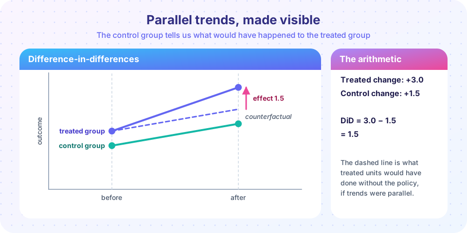
The treated group's change ΔT mixes the treatment effect with whatever else changed in that period. The control group's change ΔC estimates that "whatever else". Subtract:
DiD = ΔT − ΔC = [Ȳ(T, post) − Ȳ(T, pre)] − [Ȳ(C, post) − Ȳ(C, pre)]
In the picture above, the treated group rises from 4 to 7 (+3), the control from 3 to 4.5 (+1.5), so the DiD is 3 − 1.5 = 1.5. The difference in levels before the policy (4 versus 3) is allowed: DiD removes any constant gap between groups. That is the advantage over a simple cross-section comparison. Taking differences over time also removes the common shock, the advantage over a simple before-and-after comparison.
The regression form
With individual-level data, run
yit = α + β1 Treati + β2 Postt + δ (Treati × Postt) + εit
where Treati indicates membership in the treated group and Postt indicates the period after treatment starts. The interaction coefficient δ is the DiD estimate. With many groups and periods, the standard version uses unit and time fixed effects (chapter 7):
yit = αi + λt + δ Dit + εit, where Dit = 1 when unit i is treated in period t.
This two-way fixed effects (TWFE) regression gives the same answer as the 2×2 formula in the simple case and extends naturally to controls. Standard errors must be clustered at the level at which treatment is assigned (for example, the state), because outcomes within a unit are correlated over time, and ignoring this makes standard errors far too small (Bertrand, Duflo and Mullainathan, 2004).
The identifying assumption: parallel trends
DiD is credible if, in the absence of treatment, the treated group would have followed the same change as the control group. This is a statement about an unobservable counterfactual and cannot be proven. What you can do is gather evidence.
- Plot the pre-treatment trends. If treated and control outcomes moved together for several periods before the policy, parallel trends is more plausible. If they were already diverging, it is not.
- Run an event study. Estimate effects for each period relative to the one just before treatment. The pre-treatment coefficients should be close to zero. This is evidence, not proof: it can be low-powered, and trends can diverge exactly when treatment starts.
- Placebo tests. Apply the same estimator to an outcome that cannot be affected by the treatment, or to a fake treatment date in the pre-period, and check that the estimated effect is zero.
- Think about threats. Is the policy adopted because of a shock that hits the treated area? Did people anticipate it and change behaviour early (anticipation)? Did the composition of the groups change (people moving)? Are other policies introduced at the same time?
Parallel trends is sensitive to the functional form. Trends can be parallel in levels but not in logs, so the choice of outcome transformation is part of the assumption.
Doing it in code
First the 2×2 case. We simulate four group-period cells with a true effect of 1.5, estimate the DiD from group means and from the regression, and then show what happens when the groups were already on different trends.
Press Run (or Ctrl + Enter) to see the result here.
Program input · what you'd type while the program runs
Type the answers before you press Run, one per line. Each time the program reads a line (with input()), it gets the next line from this box.
The two computations agree exactly: the interaction coefficient is the difference of differences. When parallel trends fail, DiD simply attributes the extra trend to the policy and overstates the effect by the amount of the extra trend.
An event study
An event study estimates one coefficient per period, relative to a base period. The code builds a panel of 200 units over 12 periods, treats half of them starting at period 7, and recovers the effect period by period. In the simulated world there is no anticipation and the effect builds up over time.
Press Run (or Ctrl + Enter) to see the result here.
Program input · what you'd type while the program runs
Type the answers before you press Run, one per line. Each time the program reads a line (with input()), it gets the next line from this box.
The pre-treatment points should hover around zero (parallel trends) and the post-treatment points should rise, tracing the effect that was built in. Reading a real event study works the same way: you look at whether the pre-period is flat before reading the post-period.
Staggered adoption and modern developments
Often treatment starts at different times in different units (states adopt a law in different years). Recent research (Goodman-Bacon, 2021; Callaway and Sant'Anna, 2021; Sun and Abraham, 2021; de Chaisemartin and D'Haultfœuille, 2020) showed that the standard TWFE regression can mislead in this setting when effects change over time or differ across groups: it implicitly uses already-treated units as controls for later-treated ones and can even assign negative weights to some comparisons. The modern remedy is to estimate group-time effects with only clean comparisons (not-yet-treated or never-treated units as controls) and then aggregate. If your treatment timing is staggered, use one of these estimators or at least examine the decomposition before trusting TWFE.
Common misconceptions
"Parallel pre-trends prove the assumption." They support it. The assumption concerns the post-treatment counterfactual, which we never observe.
"DiD requires treated and control groups to be identical." It requires only that their changes would have been the same. A constant level gap is fine.
"With many units I do not need to cluster." Cluster by the level of treatment assignment; the number of clusters, not units, drives reliability.
"Two-way fixed effects always equals DiD." It does in the 2×2 case; with staggered timing and heterogeneous effects it can be biased.
Check your understanding
Quick check · 5 questions
of 5 answered You scored / 5 · perfect!
-
1. Treated outcomes rise from 10 to 16; control outcomes rise from 8 to 11. The DiD estimate is...
(16 - 10) - (11 - 8) = 6 - 3 = 3. -
2. In the regression y = a + b1 Treat + b2 Post + d (Treat x Post), which coefficient is the DiD estimate?
The interaction coefficient measures the extra change for the treated group in the post period. -
3. The parallel-trends assumption says that without treatment...
It is about changes, not levels. -
4. Event-study coefficients before the treatment date that are far from zero suggest...
A pre-trend means the groups were already diverging, which undermines the comparison. -
5. Why cluster standard errors by the unit of treatment assignment in DiD?
Serial correlation within units makes conventional standard errors too small.
Summary
- DiD estimates the effect as the change in the treated group minus the change in the control group; the regression interaction gives the same number.
- Its identifying assumption is parallel trends; support it with pre-trend plots, event studies and placebo tests.
- Cluster standard errors at the level of treatment assignment.
- With staggered adoption, prefer modern group-time estimators over naive two-way fixed effects.
Next: Regression discontinuity
Track your progress
Create a free account to tick off lessons and pick up where you left off on any device.
of Econometrics lessons completed