


















Lesson 45 of 49 · Projects and Practice
Project: returns to schooling with an instrument
A hands-on IV project with simulated data: compare OLS and 2SLS, check strength and validity, test endogeneity and quantify how far a flawed instrument can mislead.
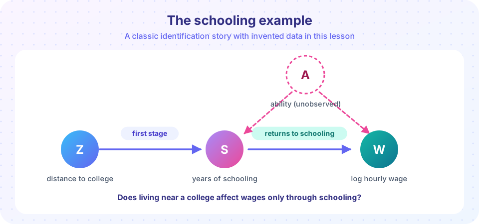
Few questions in economics have drawn as much effort as this one: what is the causal effect of an extra year of schooling on earnings? OLS gives a number, but ability, family background and ambition influence both how long people study and how much they earn, so the OLS number is probably too high. Researchers have tried to get around the problem with instruments: variables that push people toward more or less schooling for reasons unrelated to their ability. Classic choices include distance to the nearest college, local tuition and compulsory-schooling laws.
In this project you will run the complete IV analysis from chapter 6 on a simulated data set in which you know the truth. That lets you see what each diagnostic does, and, in the last step, what a subtle violation of the exclusion restriction does to the answer.
What you will learn
- How to organize an IV project: OLS, first stage, reduced form, 2SLS and tests.
- How to report strength, validity and endogeneity diagnostics together.
- How to quantify the sensitivity of IV to a small violation of the exclusion restriction.
- How to write up an IV result with its caveats.
Key terms
Instrument Z: here, distance to the nearest college (in tens of miles) and local tuition (in hundreds of dollars). Control W: a variable included in both stages, here a measure of parental education. Plausible exogeneity: a sensitivity analysis asking how big a direct effect γ of the instrument on the outcome would overturn the result. Return to schooling: the percentage change in wages per extra year of education.
The setting and the plan
The simulated world: ability A is unobserved, raises schooling and raises wages directly. Living far from a college and high local tuition both reduce schooling but are unrelated to ability by construction. The true return to a year of schooling is 0.08. Parental education is observed, raises schooling and wages, and is a control in every regression.
The plan, in order:
- OLS of log wage on schooling and the control.
- First stage: schooling on both instruments and the control; report the F statistic for the instruments.
- Reduced form: log wage directly on the instruments; the instruments should predict wages.
- 2SLS with robust standard errors; compare with OLS.
- Overidentification (Hansen J) and endogeneity (Hausman) tests.
- Sensitivity to a flawed exclusion restriction.
Steps 1 to 5
Press Run (or Ctrl + Enter) to see the result here.
Program input · what you'd type while the program runs
Type the answers before you press Run, one per line. Each time the program reads a line (with input()), it gets the next line from this box.
Interpret each line the way you would in a paper. OLS overstates the return because ability pushes both variables. The first-stage F is far above 10 and the instruments have the expected negative signs. The reduced form shows that distance and tuition reduce wages, which is what the story predicts (through schooling). The 2SLS estimate should be close to 0.08, with a larger standard error than OLS. Hansen J should not reject, and the Hausman statistic should be large, confirming that OLS is biased.
Note the rough check at the end: the Wald ratio with distance alone gives a similar answer (without controls, so a little noisier); the two instruments tell a consistent story, which is what J is formally testing.
Reading the numbers like a referee
A referee would look at four things before believing the 2SLS number. First, the sign and size of the first-stage coefficients: they should match the story (more distance and higher tuition mean less schooling) and be large enough that the instruments clearly matter. Second, the reduced form: if the instruments do not predict wages at all, no clever scaling will rescue the analysis. Third, the gap between OLS and 2SLS: its direction should agree with what theory predicts for the omitted variable, and a very large gap in the wrong direction should prompt a search for a problem. Fourth, the standard error: 2SLS is noisier than OLS, so the interval will be wider. A reader should be able to see whether the plausible range of the true return is narrow enough to be useful. Notice also what is held fixed in each column of your table, because comparing OLS with controls to IV without them would muddle the comparison.
Step 6: what if the exclusion restriction is slightly wrong?
The most important diagnostic of all cannot be run on real data, but a sensitivity analysis can show how fragile your conclusion is. Suppose distance has a direct effect γ on log wages, perhaps because people who live far from colleges live in areas with fewer high-paying jobs. Then the simple IV estimate converges to
β_IV ≈ β + γ / π
where π is the first-stage slope of schooling on the instrument. The weaker the first stage (small π), the more a small γ is magnified. The simulation below adds a direct effect of distance on wages and shows the IV estimate for several values of γ.
Press Run (or Ctrl + Enter) to see the result here.
Program input · what you'd type while the program runs
Type the answers before you press Run, one per line. Each time the program reads a line (with input()), it gets the next line from this box.
With a first-stage slope around −0.35, each 0.01 of direct effect moves the IV estimate by about 0.03 in absolute value. Compared with a true return of 0.08, a seemingly tiny direct effect can overturn the result. That is why the exclusion restriction deserves paragraphs, not a footnote.
Writing up the result
A good write-up has the following elements.
- The question and the instrument, with the argument for exclusion in words: why distance to college should not affect wages other than through schooling, and what could make that false (local labour markets, family sorting).
- A table with OLS, reduced form, first stage and 2SLS columns, the first-stage F, and the Hansen J p-value.
- A comparison of OLS with IV and an explanation of the direction of the difference.
- A sensitivity statement: how large a direct effect would overturn the conclusion.
- Scope: the estimate applies to people whose schooling is moved by distance and tuition, the compliers (LATE).
Your turn
- Make the instruments weak (shrink the coefficients on
distandtuitionto 0.05) and watch F, the 2SLS estimate and its standard error. - Make tuition invalid by adding
0.1 * Ato it (richer, more able areas have higher tuition). Does Hansen J detect it? Does the estimate move? - Replace the single control with several and check that the 2SLS estimate remains stable.
- Compute a 95% interval for the IV estimate and for OLS. Do they overlap?
Common misconceptions
"If J does not reject, my instruments are valid." J tests agreement among instruments. If both share a flaw, they agree and J passes.
"A bigger sample makes IV safe." A larger sample shrinks the standard error but not the bias from an invalid instrument.
"IV gives the return to schooling for everyone." It estimates the effect for people whose schooling is moved by the instrument.
Check your understanding
Quick check · 5 questions
of 5 answered You scored / 5 · perfect!
-
1. In this project, why is the OLS return to schooling too high?
Positive correlation between schooling and the omitted ability term biases the slope upward. -
2. The simple IV estimate with a direct effect gamma of the instrument on the outcome converges to...
The direct effect contaminates the reduced form; dividing by the first-stage slope pi gives beta + gamma / pi. -
3. With a weaker first stage (smaller pi), a given direct effect gamma produces...
The bias gamma / pi grows as pi shrinks. -
4. Which result would most strongly suggest that OLS was biased here?
A large difference between IV and OLS, supported by the Hausman test, indicates endogeneity. -
5. The IV estimate in this project applies to...
IV identifies a LATE for compliers.
Summary
- An IV project runs OLS, the first stage (with F), the reduced form, 2SLS with robust SEs, then J and Hausman tests.
- IV removes the ability bias but widens the standard errors and speaks only for compliers.
- The bias from a direct effect of the instrument is about
γ / π: weak first stages amplify small violations. - Write up the argument for exclusion, the diagnostics and the sensitivity analysis together.
Track your progress
Create a free account to tick off lessons and pick up where you left off on any device.
of Econometrics lessons completed