


















Lesson 21 of 49 · Inference and Specification
Specification, omitted variables and multicollinearity
Understand omitted variable bias and its direction, irrelevant variables, multicollinearity and the variance inflation factor, bad controls and measurement error, with runnable simulations.
A specification is a decision: which variables to include, in what form, and which to leave out. The classical results of the last lessons hold only if the specification is right, in the sense that MLR.4 holds: nothing left in the error term is related to the regressors. Real models are never perfect, so the practical question is how wrong specification harms estimates, in which direction, and how to detect it.
This lesson studies the most important specification problems: leaving out a relevant variable (bias), including irrelevant ones (extra noise), including variables that are nearly redundant (multicollinearity), including the wrong kinds of controls and measuring a variable with error. For each one you will learn what happens and what to do.
What you will learn
- The omitted variable bias formula and how to sign the bias.
- Why irrelevant variables do not bias but do add variance.
- What multicollinearity does, and how to read the variance inflation factor.
- Which controls to avoid, and what measurement error does to a slope.
Key terms
Omitted variable bias: the bias in a slope caused by leaving out a variable that affects y and is correlated with the included regressor.
Confounder: a variable that influences both the regressor of interest and the outcome.
Multicollinearity: strong correlation among regressors, making individual coefficients imprecise.
Variance inflation factor (VIF): 1/(1 − Rj²), the factor by which collinearity inflates the variance of bj.
Attenuation bias: shrinkage of a slope toward zero caused by measurement error in the regressor.
Omitted variable bias
Suppose the true model is
wage = β0 + β1·educ + β2·ability + u
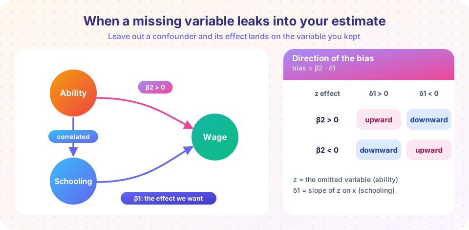
but ability is unmeasured, so you regress wage on schooling alone. The regression's slope b̃1 is not an estimate of β1. From the algebra in the multiple regression lesson, in expectation
E[b̃1] = β1 + β2 · δ1
where δ1 is the slope you would get from regressing the omitted variable (ability) on the included one (schooling). The second term, β2·δ1, is the omitted variable bias. It is zero only if (a) the omitted variable does not affect y (β2 = 0) or (b) it is uncorrelated with the included regressor (δ1 = 0). Both conditions must be failed for a bias to arise: the omitted variable must matter and move with x.
Signing the bias
You usually cannot measure the omitted variable, but you can reason about the direction of the bias from the sign of β2 and the sign of δ1:
δ1 > 0 (corr(x, z) positive) |
δ1 < 0 (corr(x, z) negative) |
|
|---|---|---|
β2 > 0 (z raises y) |
upward bias | downward bias |
β2 < 0 (z lowers y) |
downward bias | upward bias |
Example: ability raises wages (β2 > 0) and more able people tend to get more schooling (δ1 > 0), so the bias is upward: the naive wage-schooling slope overstates the return to schooling because it picks up some of ability's effect. If instead the omitted variable were "family obligations that reduce hours worked" and it was more common among people with less schooling, the sign analysis would differ: work through it using the table.
This is the standard "direction of bias" argument that referees expect in empirical papers. It does not fix the bias, but it tells readers whether your estimate is an over- or under-estimate and thus how to read the sign and size.
What to do
- Include the variable if you can measure it (or a good proxy, such as a test score for ability).
- Use a different design if you cannot: instrumental variables (Chapter 6), panel fixed effects (Chapter 7), difference-in-differences or regression discontinuity (Chapter 8).
- Be honest: report the likely direction of the remaining bias.
Irrelevant variables
Including a variable whose true coefficient is zero does not bias the other slopes. OLS remains unbiased because the true model is still nested. But the cost is precision: the extra regressor uses up a degree of freedom and, if correlated with the others, reduces the independent variation in them, raising their variances. In small samples the loss can matter. The rule is asymmetric: omitting a relevant variable biases; including an irrelevant one adds noise. When in doubt about a relevant confounder, include it.
Multicollinearity
Recall the variance of a slope in multiple regression:
Var(bj) = σ² / [ SSTj · (1 − Rj²) ]
Here SSTj is the total variation in xj and Rj² is the R-squared from regressing xj on the other regressors. The factor 1/(1 − Rj²) is the variance inflation factor, VIF. If xj is almost a linear function of the others (Rj² close to 1), the VIF is huge and so is the variance.
Rj² |
VIF | Standard error multiplied by |
|---|---|---|
| 0 | 1 | 1 |
| 0.5 | 2 | 1.41 |
| 0.9 | 10 | 3.16 |
| 0.99 | 100 | 10 |
So with Rj² = 0.9 the standard error is about 3.2 times larger than if the regressor were uncorrelated with the others. Rules of thumb flag a VIF above 10 as worrying, but treat that threshold as a prompt to look closer, not as a law.
What multicollinearity does and does not do
It does inflate standard errors, make coefficients sensitive to small changes in the sample or specification, and produce individually insignificant coefficients in a jointly significant model (Lesson 3's F-test point). It does not bias estimates, violate MLR.1 to MLR.5 (only perfect collinearity violates MLR.3), or affect predictions made within the range of the data.
What to do about it
- Nothing, if your variable of interest is not collinear with the others: collinearity among control variables does not harm the estimate of the variable you care about.
- Collect more data, or more variation, which attacks the root cause.
- Combine variables into an index or drop one of two near-duplicates, if substantive reasoning supports it.
- Test jointly with an F test rather than relying on individual t statistics.
Dropping a relevant variable just to reduce collinearity trades a variance problem for a bias problem, usually a bad bargain.
Which controls to include
More controls are not always better. Include variables that are confounders: they affect both the regressor and the outcome. Be careful with:
- Mediators. If schooling raises wages by raising job type, then controlling for job type removes part of the effect you are trying to measure.
- Consequences of the outcome. Controlling for a variable that is itself caused by
ycan create bias (a "collider" or reverse causation).
The decision comes from the causal story, not from statistical fit. A higher R-squared never justifies adding a variable.
Functional form misspecification
Leaving out a squared term when the relationship is curved is an omitted variable problem in disguise: the missing x² is correlated with x. Plot the residuals against the regressors and the fitted values and look for a pattern. A formal check, the RESET test, adds powers of the fitted values (such as ŷ² and ŷ³) to the regression and tests them jointly with an F test. A significant result suggests the functional form is misspecified, though it does not say how to repair it.
Measurement error
If the regressor you observe is a noisy version of the true one (x = x* + e, with e independent noise), OLS slopes are biased toward zero, the attenuation bias:
plim b1 = β1 · Var(x*) / [ Var(x*) + Var(e) ]
The factor is the reliability ratio, the share of the observed variation that is true signal. If 80% of the variance of your measure is signal, the estimated slope is only 80% of the truth, however large the sample. Measurement error in the dependent variable, by contrast, does not bias slopes (it raises the error variance and reduces precision). Instrumental variables, covered in Chapter 6, are the classic remedy for noisy regressors.
Common misconceptions
"Omitted variable bias disappears in large samples." It does not. The bias is a property of the specification, not of the sample size.
"Multicollinearity biases estimates." It inflates variances but leaves OLS unbiased.
"Add every variable you can; more controls are safer." Mediators and consequences of the outcome can introduce bias.
"Measurement error only adds noise." Error in a regressor biases its slope toward zero.
Try it
First example: simulate omitted variable bias. The true effect of x is 1.0; a hidden z affects y and is correlated with x. We compare the short regression with the prediction β1 + β2·δ1 and with the long regression that includes z.
Press Run (or Ctrl + Enter) to see the result here.
Program input · what you'd type while the program runs
Type the answers before you press Run, one per line. Each time the program reads a line (with input()), it gets the next line from this box.
Second example: multicollinearity. We keep the true model fixed and make the two regressors increasingly correlated, measuring the standard deviation of the slope on x1 across many repeated samples. The theoretical inflation is √VIF.
Press Run (or Ctrl + Enter) to see the result here.
Program input · what you'd type while the program runs
Type the answers before you press Run, one per line. Each time the program reads a line (with input()), it gets the next line from this box.
Third example: attenuation bias from measurement error. The true slope is 2. We observe x with noise whose variance is one quarter of the true variance, so the reliability ratio is 0.8.
Press Run (or Ctrl + Enter) to see the result here.
Program input · what you'd type while the program runs
Type the answers before you press Run, one per line. Each time the program reads a line (with input()), it gets the next line from this box.
Check your understanding
Quick check · 5 questions
of 5 answered You scored / 5 · perfect!
-
1. Omitted variable bias requires that the omitted variable
The bias is β2·δ1, which is nonzero only if the omitted variable matters (β2 ≠ 0) and moves with x (δ1 ≠ 0). -
2. Ability raises wages and is positively correlated with schooling. Omitting ability makes the schooling slope
β2 > 0 and δ1 > 0, so the bias β2·δ1 is positive. -
3. Including an irrelevant variable in a regression
The true model is still nested, so OLS stays unbiased, but precision can suffer. -
4. If Rj² = 0.9, the variance inflation factor for xj is
VIF = 1/(1 − 0.9) = 10. -
5. Classical measurement error in a regressor biases its slope
The slope is multiplied by the reliability ratio, which is less than 1.
Summary
- Omitting a relevant variable correlated with the regressor biases the slope by
β2·δ1; sign it using the signs ofβ2andδ1. - Including irrelevant variables does not bias but costs precision.
- Multicollinearity inflates variances by the VIF
1/(1 − Rj²)without causing bias. - Control for confounders, not for mediators or consequences of the outcome.
- Measurement error in a regressor attenuates its slope toward zero by the reliability ratio.
Next: Chapter 4 review
Track your progress
Create a free account to tick off lessons and pick up where you left off on any device.
of Econometrics lessons completed