


















Lesson 30 of 49 · Instrumental Variables and Endogeneity
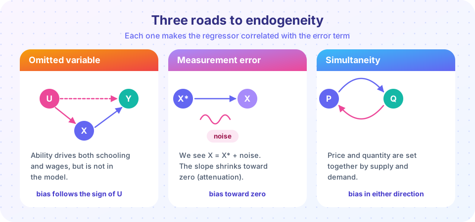
Three roads to endogeneity
Learn the three classic sources of endogeneity, derive the direction of the bias in each, and verify every formula with a simulation in Python.
Every IV analysis starts with a diagnosis: why do we think the regressor is correlated with the error? The answer shapes both the instrument we search for and the direction in which we expect OLS to be wrong. Econometrics textbooks sort the causes into three families. This lesson takes each in turn, derives the bias, and checks it with a simulation.
What you will learn
- The omitted-variable bias formula and how to sign the bias.
- Why classical measurement error in a regressor shrinks the slope toward zero, but error in the outcome does not.
- Why simultaneous determination makes price regressions meaningless without more structure.
- How to ask "what is in my error term?" for any regression.
Key terms
Omitted variable bias (OVB): bias from leaving out a variable that affects y and is correlated with an included regressor. Classical measurement error: observed x = x* + v, with noise v uncorrelated with the truth. Attenuation bias: shrinkage of a slope toward zero. Reliability ratio: Var(x*) / (Var(x*) + Var(v)). Simultaneity: two or more variables determined jointly, each in the other's equation.
Road 1: omitted variables
Suppose the true model is y = β0 + β1x + β2a + u, but you cannot observe a (say, ability) and so regress y on x alone. Your error is now β2a + u, and it is correlated with x whenever a and x are. How far off is OLS? Define the auxiliary relation a = δ0 + δ1x + (noise), where δ1 = Cov(x, a) / Var(x). Then in large samples
plim b1 = β1 + β2 δ1
The bias is the product of two things: the effect of the omitted variable on y (β2) and the association between the omitted and included variables (δ1). That gives the familiar sign table.
δ1 > 0 (x and a move together) |
δ1 < 0 |
|
|---|---|---|
β2 > 0 |
upward bias | downward bias |
β2 < 0 |
downward bias | upward bias |
Schooling and ability: both β2 (ability raises wages) and δ1 (able people get more schooling) are positive, so OLS overstates the return to schooling. This sign reasoning is useful even when you cannot estimate the bias, because it tells you whether your result is likely a lower bound or an upper bound.
Adding the omitted variable fixes the problem only if you can measure it. Control variables help but cannot remove unobserved confounders, which is the reason for instruments.
Road 2: measurement error
Data are never perfectly measured: survey respondents misreport income, price indices are approximations, "years of experience" is usually a guess. Two cases behave very differently.
Error in the dependent variable. If you observe y = y* + e and the noise e is unrelated to the regressors, it simply joins the error term. The slopes stay unbiased and only precision suffers.
Error in a regressor (classical errors-in-variables). If you observe x = x* + v, with v uncorrelated with x* and u, and the true model is y = β0 + β1x* + u, then the model you can estimate is y = β0 + β1x + (u − β1v). The regressor x is correlated with the composite error through v. A short calculation gives
plim b1 = β1 × Var(x*) / (Var(x*) + Var(v)) = β1 × λ
with λ the reliability ratio, between 0 and 1. The estimated slope is attenuated toward zero: noisier measurement means a bigger shrinkage. If half of the observed variance of x is noise, you estimate half the true effect. With several regressors the bias is not as simple: the error in one variable contaminates the others too, and signs can flip.
An instrument can undo attenuation: a second, independent measurement of the same quantity (for example, a second survey report) is correlated with the truth and with the first measurement, but its error is unrelated to the first one's error.
Road 3: simultaneity
Quantities and prices are the textbook case. Suppose
Demand: Q = a − b P + uD
Supply: Q = c + d P + uS
with b, d > 0. In equilibrium both equations hold at once, so the price is a function of both shocks: P = (a − c + uD − uS) / (b + d). A demand shock uD pushes the price up, so P is positively correlated with uD, the error of the demand equation. Regressing Q on P mixes up two curves: you get a blend of the demand slope and the supply slope, not the demand slope. With equal shock variances, the OLS slope estimates −b + (b + d)/2 = (d − b)/2, so with b = 2, d = 3 the regression of quantity on price returns a positive number even though demand slopes down.
Simultaneity is not restricted to markets: crime and police, income and consumption, and a country's growth and its investment all involve feedback. The remedy is a variable that shifts one of the equations without appearing in the other. A supply shifter such as the cost of an input moves the supply curve along a stable demand curve and traces out the demand slope.
Simulating omitted variables
The code compares the "short" regression (leaving out ability) and the "long" regression, and checks the formula β1 + β2 δ1.
Press Run (or Ctrl + Enter) to see the result here.
Program input · what you'd type while the program runs
Type the answers before you press Run, one per line. Each time the program reads a line (with input()), it gets the next line from this box.
The short slope should match β1 + β2δ1 closely (the sample is huge), while the long slope should sit close to the true 0.10. Notice that with a positive δ1 and positive β2, the short slope overshoots.
Simulating attenuation
Press Run (or Ctrl + Enter) to see the result here.
Program input · what you'd type while the program runs
Type the answers before you press Run, one per line. Each time the program reads a line (with input()), it gets the next line from this box.
The dots follow the curve β × Var(x*) / (Var(x*) + Var(v)). With noise standard deviation 1, equal to the standard deviation of the truth, the slope is cut roughly in half.
Simulating simultaneity
Press Run (or Ctrl + Enter) to see the result here.
Program input · what you'd type while the program runs
Type the answers before you press Run, one per line. Each time the program reads a line (with input()), it gets the next line from this box.
OLS returns something that is neither the demand slope nor the supply slope. The cost shifter w moves only the supply curve, so using it as an instrument recovers the demand slope, close to −2.
A habit: interrogate your error term
For any regression, write down what is inside the error and ask which parts could be related to your regressor. If you can name a plausible driver (ability, local conditions, unobserved quality) and tell a story about the sign, you have both a diagnosis and an expectation for the bias. If you cannot think of any, the regression may be safe, but the burden is on you to argue it.
Common misconceptions
"Measurement error always biases toward zero." That holds for classical error in a single regressor. With several mismeasured regressors, or errors correlated with the truth, the direction can differ.
"Adding more controls always removes endogeneity." Controls help only for confounders you can measure. Adding "bad controls" (variables affected by the regressor) can even create bias.
"Simultaneity is just reverse causality, and a lag solves it." Lagging the regressor can help with timing, but if shocks persist or agents anticipate, the lag is still endogenous.
Check your understanding
Quick check · 5 questions
of 5 answered You scored / 5 · perfect!
-
1. A researcher omits a variable that is positively related to both y and the included regressor x. The bias in the slope of x is...
plim b1 = beta1 + beta2 * delta1 with both terms positive, so the slope is overstated. -
2. Classical measurement error in the dependent variable...
The noise is absorbed into the error term and is unrelated to the regressors. -
3. The reliability ratio of a regressor is 0.6. The OLS slope converges to what share of the true slope?
plim b1 = lambda times beta1, so 0.6 of the true value. -
4. In a supply and demand system, why is price endogenous in the demand equation?
The equilibrium price depends on the demand shock, so it is correlated with the demand error. -
5. Which variable is a good instrument for the demand slope?
A supply shifter moves the equilibrium along the demand curve, tracing out its slope.
Summary
- Omitted variables bias the slope by
β2 δ1; the signs of the two parts tell you the direction. - Classical measurement error in a regressor attenuates the slope by the reliability ratio; error in
yonly adds noise. - Simultaneity makes price (or any jointly determined variable) correlated with the error; a shifter of the other equation identifies the slope.
- Ask "what is in my error term?" before you reach for an instrument.
Next: Two-stage least squares
Track your progress
Create a free account to tick off lessons and pick up where you left off on any device.
of Econometrics lessons completed