


















Lesson 12 of 49 · Simple and Multiple Regression
Simple linear regression and OLS
Derive the ordinary least squares slope and intercept, work a five-point example by hand, interpret coefficients and units, and learn the properties residuals must satisfy.
The simplest regression has one outcome y and one explanatory variable x. You believe, or at least want to summarize, that y changes in a roughly straight-line way with x, plus noise. The population model is
y = β0 + β1 · x + u
where β0 is the intercept, β1 the slope and u the disturbance (everything else). The Greek letters are unknown population parameters. Your sample gives you estimates b0 and b1 (also written β̂0 and β̂1), and the fitted line ŷ = b0 + b1·x. This lesson explains where the OLS formulas come from, how to compute them by hand and what they mean.
What you will learn
- How OLS defines the best line through the sum of squared residuals.
- The slope and intercept formulas and what they say in words.
- How to compute and interpret an OLS line by hand.
- The algebraic properties that residuals always satisfy.
Key terms
Fitted value ŷi = b0 + b1·xi: the line's prediction for observation i.
Residual ûi = yi − ŷi: the gap between the observation and the line.
Sum of squared residuals (SSR): Σ ûi², the quantity OLS minimizes.
Intercept b0: the predicted y when x = 0.
Slope b1: the predicted change in y per one-unit increase in x.
The least squares idea
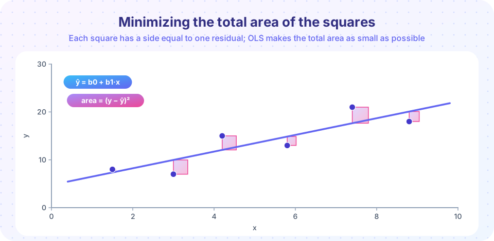
Draw any line through a cloud of points and measure, for each point, the vertical distance to the line. Some points lie above (positive residual), some below (negative). Add the residuals and the positives cancel the negatives, which is useless for judging fit, since a bad line can have residuals that sum to zero. Squaring first removes the sign and punishes large misses more than small ones. OLS therefore picks b0 and b1 to make
SSR(b0, b1) = Σ (yi − b0 − b1·xi)²
as small as possible.
Why squares and not absolute values? Squaring leads to clean formulas (and, with certain assumptions, to the best possible estimator, as you will see in Chapter 4), and it connects the line to averages: the mean is the number that minimizes squared deviations, just as OLS is the line that minimizes squared residuals.
Deriving the formulas
You can minimize SSR with calculus: set its derivatives with respect to b0 and b1 to zero. This gives two equations, the normal equations:
Σ (yi − b0 − b1·xi) = 0                 (1)
Σ xi · (yi − b0 − b1·xi) = 0            (2)
The first says residuals sum to zero. Solving it for b0 gives b0 = ȳ − b1·x̄: the line passes through the point of means (x̄, ȳ). Substituting into (2) and simplifying yields
b1 = Σ (xi − x̄)(yi − ȳ) / Σ (xi − x̄)²  =  Cov(x, y) / Var(x)
b0 = ȳ − b1 · x̄
The slope has a clear interpretation: it is the covariance of x and y divided by the variance of x. It takes the co-movement of the two variables and scales it by how much x moves in the first place. If x and y are uncorrelated, b1 = 0 and the best line is flat at ȳ. The estimates exist whenever x varies (Var(x) > 0); if every observation has the same x, you cannot say how y changes with x.
A complete worked example
Take five invented observations: x = 1, 2, 3, 4, 5 and y = 1, 3, 2, 5, 4.
Step 1, means: x̄ = 3, ȳ = 3.
Step 2, deviations:
| i | x | y | x − x̄ | y − ȳ | (x − x̄)(y − ȳ) | (x − x̄)² |
|---|---|---|---|---|---|---|
| 1 | 1 | 1 | −2 | −2 | 4 | 4 |
| 2 | 2 | 3 | −1 | 0 | 0 | 1 |
| 3 | 3 | 2 | 0 | −1 | 0 | 0 |
| 4 | 4 | 5 | 1 | 2 | 2 | 1 |
| 5 | 5 | 4 | 2 | 1 | 2 | 4 |
| Sum | 8 | 10 |
Step 3, slope and intercept: b1 = 8 / 10 = 0.8 and b0 = 3 − 0.8 × 3 = 0.6. The fitted line is ŷ = 0.6 + 0.8x.
Step 4, fitted values and residuals: the fitted values are 1.4, 2.2, 3.0, 3.8, 4.6. The residuals y − ŷ are −0.4, 0.8, −1.0, 1.2, −0.6.
Step 5, checks: the residuals sum to −0.4 + 0.8 − 1.0 + 1.2 − 0.6 = 0, as normal equation (1) requires. The sum of squared residuals is 0.16 + 0.64 + 1.00 + 1.44 + 0.36 = 3.60. Try any other line, such as ŷ = 1 + 0.7x, and its SSR will be larger.
Interpreting the coefficients
In the model wage = β0 + β1·educ, with wage in dollars per hour and educ in years, an estimate b1 = 1.07 means: workers with one more year of schooling earn, on average, $1.07 more per hour in this sample. Notice four features of a good interpretation.
- Units. Always state both. "Dollars per hour per year of schooling."
- Comparison, not intervention. The coefficient compares groups that differ by one unit of
x. It does not (yet) say what would happen to one person who gets another year. - Association, not necessarily causation. Whether the number is a causal effect depends on whether
uis related tox(Chapters 4 and 6). - Range of the data. The intercept
b0predictsyatx = 0. If no observation hasxnear zero,b0is an extrapolation and often meaningless on its own. It anchors the line, nothing more.
Changing units
Rescaling changes coefficients in predictable ways, which is a handy check on your work. If you measure wages in cents instead of dollars, y is multiplied by 100 and so are b0 and b1. If you measure schooling in months instead of years, x is multiplied by 12 and b1 is divided by 12, while b0 and the fitted values are unchanged. The fit does not depend on units; only the labels on the coefficients do.
Properties of OLS residuals
These follow from the normal equations and hold for every OLS fit with an intercept, in every data set, no matter how bad the model:
- The residuals sum to zero, so their mean is zero.
- The residuals are uncorrelated with
xin the sample:Σ xi·ûi = 0. - The residuals are uncorrelated with the fitted values.
- The line passes through
(x̄, ȳ).
Because of these, you cannot check the model's assumptions simply by confirming the residuals look uncorrelated with x; they always do. That is a property of the method, not evidence about the truth. What you can do is plot residuals against x and the fitted values to look for patterns such as curves or changing spread, which we do in Chapters 4 and 5.
Common misconceptions
"The slope is the effect of x on y." The slope is the association in your data. It equals the causal effect only under conditions you must defend.
"The residual û is the same as the error u." The error u is unobserved and belongs to the population model. The residual û is computed from your estimated line. They are related but different, much as the sample mean differs from the population mean.
"A larger slope means a stronger relationship." Slope depends on units. A strong relationship can have a tiny slope if x is measured in large units. Use correlation or R-squared for strength.
Try it
First example: do the hand calculation by computer, and verify both the formulas and the residual properties. Everything printed in the last three lines should be zero (up to rounding).
Press Run (or Ctrl + Enter) to see the result here.
Program input · what you'd type while the program runs
Type the answers before you press Run, one per line. Each time the program reads a line (with input()), it gets the next line from this box.
Second example: change units and watch the coefficients change while the fit does not. We use invented hourly wages and years of schooling.
Press Run (or Ctrl + Enter) to see the result here.
Program input · what you'd type while the program runs
Type the answers before you press Run, one per line. Each time the program reads a line (with input()), it gets the next line from this box.
Third example: the residuals as a picture, drawn with the house plot style. Pink segments are the residuals; the squares of their lengths add up to the SSR that OLS minimizes.
Press Run (or Ctrl + Enter) to see the result here.
Program input · what you'd type while the program runs
Type the answers before you press Run, one per line. Each time the program reads a line (with input()), it gets the next line from this box.
Check your understanding
Quick check · 5 questions
of 5 answered You scored / 5 · perfect!
-
1. In the worked example (x = 1..5, y = 1, 3, 2, 5, 4) the OLS slope is
Σ(x − x̄)(y − ȳ) = 8 and Σ(x − x̄)² = 10, so b1 = 0.8. -
2. The OLS slope in simple regression equals
The slope scales the covariance by the variance of x. -
3. If y is measured in cents instead of dollars, the slope b1 is
y is multiplied by 100, so every coefficient in the equation for y is also multiplied by 100. -
4. Which statement is true for every OLS fit with an intercept?
These properties follow from the normal equations, whatever the data. -
5. Why is the intercept sometimes not worth interpreting?
If no observations have x near zero, the intercept is an extrapolation.
Summary
- OLS chooses
b0andb1to minimizeΣ(y − b0 − b1·x)². - The slope is
Cov(x, y)/Var(x)and the intercept isȳ − b1·x̄, so the line passes through the point of means. - Residuals sum to zero and are uncorrelated with
xby construction. - Interpret a slope with units, as a comparison across groups, and with caution about causation.
- Rescaling variables rescales coefficients but leaves the fit unchanged.
Track your progress
Create a free account to tick off lessons and pick up where you left off on any device.
of Econometrics lessons completed