


















Lesson 16 of 49 · Simple and Multiple Regression
Chapter 3 review: simple and multiple regression
Review chapter 3 of econometrics: OLS formulas, residual properties, R-squared, multiple regression, logs, quadratics and dummies, with a recap table and a ten-question quiz.
In this chapter you learned to turn a scatter of points into an equation: the least squares line, how to measure its fit, how to add more variables and how to bend it with logs, squares and dummies. Almost every empirical paper in economics uses these tools, so it is worth locking in the key formulas and, more importantly, how to read them.
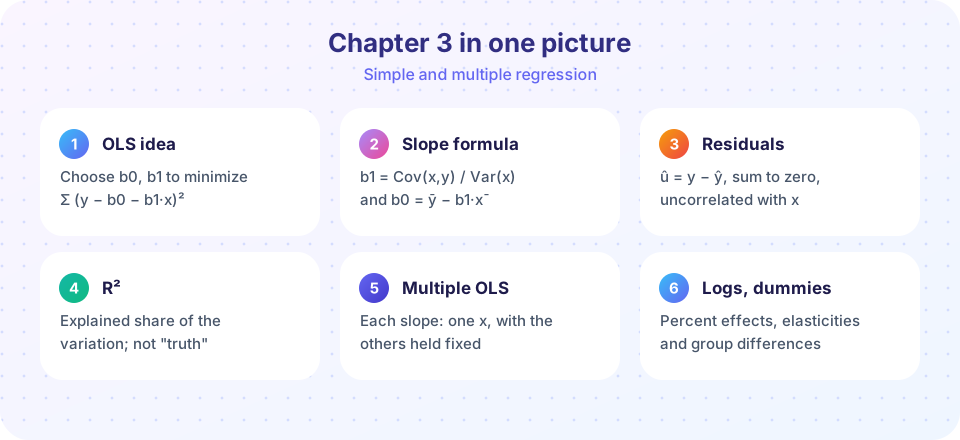
The chapter in one table
| Topic | Key formulas and facts |
|---|---|
| OLS criterion | Minimize SSR = Σ(yi − b0 − b1·xi)² |
| Simple regression | b1 = Cov(x, y)/Var(x); b0 = ȳ − b1·x̄; the line passes through (x̄, ȳ) |
| Residual properties | Σ ûi = 0; Σ xi·ûi = 0; residuals uncorrelated with fitted values |
| Fit | TSS = ESS + RSS; R² = 1 − RSS/TSS; σ̂ = √(RSS/(n − k − 1)) |
| Multiple regression | b = (X′X)⁻¹X′y; coefficient = effect holding other included variables fixed |
| Partialling out | b1 equals the slope of y on the part of x1 unexplained by other regressors |
| Slope identity | b̃1 = b1 + b2·δ1 (simple slope versus multiple slope) |
| Adjusted R² | 1 − (1 − R²)(n − 1)/(n − k − 1) |
| Log forms | log-level: 100·β percent; log-log: elasticity; level-log: β/100 units per 1% |
| Quadratic | marginal effect β1 + 2β2·x; turning point −β1/(2β2) |
| Dummies | coefficient = difference from the reference group; use m − 1 dummies |
How the pieces connect
OLS is an estimator (Chapter 2): its output is a random variable that changes with the sample. R-squared and the standard error of the regression describe how well the line fits this sample; they do not say whether the estimates are close to the truth. That question, and the question of whether a slope is causal, is the subject of Chapter 4.
Multiple regression is not magic. "Holding other things constant" is an algebraic operation, partialling out the other included variables, and it works only for variables you include and measure well. Anything left in the error term that is correlated with a regressor still contaminates the estimate.
Finally, flexible functional forms are your tool for making a linear model fit reality. Choosing the form is partly a modeling decision, guided by theory (elasticities, diminishing returns), by plots of the data and by interpretability.
Common mistakes to avoid
Interpreting a coefficient without units or without the other variables in mind. Say "holding experience constant, one more year of schooling goes with $0.90 more per hour".
Reading R-squared as validity. A model can fit well and be biased, or fit poorly and be informative.
Forgetting the dummy trap. m categories need m − 1 dummies plus an intercept.
Reading a quadratic's linear term alone. The slope depends on the level of the variable.
Mixing percent and percentage points.
Try it
First, a calculator that takes a log-level slope and reports both the approximate and the exact percentage effect, so you can see when the approximation breaks down.
Press Run (or Ctrl + Enter) to see the result here.
Program input · what you'd type while the program runs
Type the answers before you press Run, one per line. Each time the program reads a line (with input()), it gets the next line from this box.
Second, a one-stop simulation that reviews the chapter: it fits a regression with a dummy and a continuous regressor and reports the fitted coefficients, R², adjusted R² and SER, side by side with the true values.
Press Run (or Ctrl + Enter) to see the result here.
Program input · what you'd type while the program runs
Type the answers before you press Run, one per line. Each time the program reads a line (with input()), it gets the next line from this box.
Check your understanding
Quick check · 10 questions
of 10 answered You scored / 10 · perfect!
-
1. The OLS slope in simple regression equals
It is the covariance scaled by the variance of the regressor. -
2. Which property holds for every OLS fit with an intercept?
The first normal equation forces the residuals to sum to zero. -
3. If TSS = 80 and ESS = 60, then R² and RSS are
R² = 60/80 = 0.75 and RSS = TSS − ESS = 20. -
4. In ln(wage) = 2.0 + 0.10·educ, one more year of schooling goes with about
In a log-level model, 100 times the slope is the approximate percent change. -
5. In multiple regression, a coefficient describes
Each coefficient is a partial effect, ceteris paribus within the included variables. -
6. Why can adding any regressor never lower the plain R²?
OLS could set the new coefficient to zero, so the minimized SSR cannot increase. -
7. With b1 = 2.0, b2 = 0.5 and δ1 = 0.4, the simple slope of y on x1 is
b̃1 = b1 + b2·δ1 = 2.0 + 0.5 × 0.4 = 2.2. -
8. In y = b0 + b1·x + b2·x² with b1 = 4 and b2 = −0.2, the turning point is
−b1/(2·b2) = −4/(−0.4) = 10. -
9. A coefficient on a 'female' dummy of −2.0 in a wage equation (wages in dollars per hour) means
A dummy coefficient is the difference from the reference group in the outcome's units. -
10. Which describes the dummy variable trap?
The dummies sum to the intercept column, so coefficients cannot be separated.
Summary
- OLS minimizes squared residuals; the slope is
Cov(x, y)/Var(x), and the line passes through the means. R², adjustedR²and the SER describe fit, not truth, and say nothing about causation.- Multiple regression coefficients compare units alike in the other included variables, via partialling out.
- Logs give percentage and elasticity readings; quadratics give diminishing returns; dummies and interactions give group differences.
- Chapter 4 asks the next questions: when are OLS estimates unbiased, how precise are they, and how do we test hypotheses?
Track your progress
Create a free account to tick off lessons and pick up where you left off on any device.
of Econometrics lessons completed