


















Lesson 19 of 49 · Inference and Specification
t tests and confidence intervals
Learn how to test a single hypothesis about a regression coefficient with the t statistic, read p-values correctly, build confidence intervals and avoid the common misreadings of significance.
You now have an estimate and its standard error. The estimate says "schooling goes with $0.62 more per hour"; the standard error says "but this number would typically move by about $0.21 across samples". The t test and the confidence interval combine the two into a statement you can defend: is the effect distinguishable from zero (or from some other value), and what range of values is plausible?
These tools appear in every regression table in every economics paper. Used well, they keep you honest about uncertainty. Used badly, they produce false discoveries. This lesson teaches both the mechanics and the discipline.
What you will learn
- The five steps of a hypothesis test for a regression coefficient.
- How to compute and interpret a t statistic, a critical value and a p-value.
- How to build and read a confidence interval, and how it relates to the test.
- What statistical significance does and does not mean.
Key terms
Null hypothesis H0: the value you test, usually βj = 0.
Alternative H1: what holds if H0 is false: two-sided (βj ≠ 0) or one-sided (βj > 0).
Significance level α: the false rejection probability you accept, commonly 5%.
Critical value: the threshold the t statistic must exceed (in absolute value) to reject.
p-value: the smallest significance level at which you would reject; the probability under H0 of a result at least as extreme as yours.
The t statistic
To test H0: βj = c (usually c = 0), form
t = (bj − c) / se(bj)
It measures how many standard errors the estimate lies from the hypothesized value. Under MLR.1 to MLR.6 and H0, this statistic has a t distribution with n − k − 1 degrees of freedom. The t distribution looks like a normal curve with slightly heavier tails; the heaviness reflects the extra uncertainty from estimating σ with σ̂. With 30 or more degrees of freedom it is nearly normal, and as degrees of freedom grow without limit it becomes the standard normal.
The five steps
- State the hypotheses.
H0: β1 = 0againstH1: β1 ≠ 0. - Choose α, say 5%, before looking at the result.
- Compute
t = b1 / se(b1)(forc = 0). - Compare with the critical value for
n − k − 1degrees of freedom: reject if|t|exceeds it. - Report the estimate, standard error, t statistic or p-value, and a plain-language conclusion.
Typical two-sided 5% critical values: about 2.23 with 10 degrees of freedom, 2.09 with 20, 2.04 with 30, 2.00 with 60 and 1.96 in the limit. At the 1% level, they are about 2.85 with 20 degrees of freedom and 2.58 in the limit. A common rule of thumb: in a reasonably large sample, |t| > 2 is significant at roughly 5%.
Worked example 1: a small sample
For the five-point data, b1 = 0.8, se = 0.346 and there are 5 − 1 − 1 = 3 degrees of freedom. Then t = 0.8 / 0.346 ≈ 2.31. The 5% two-sided critical value for 3 degrees of freedom is 3.18, so we do not reject H0: β1 = 0, even though the slope looks sizable. With so few observations the t distribution is very heavy-tailed; the data are simply too few to distinguish this slope from zero.
Worked example 2: a typical regression
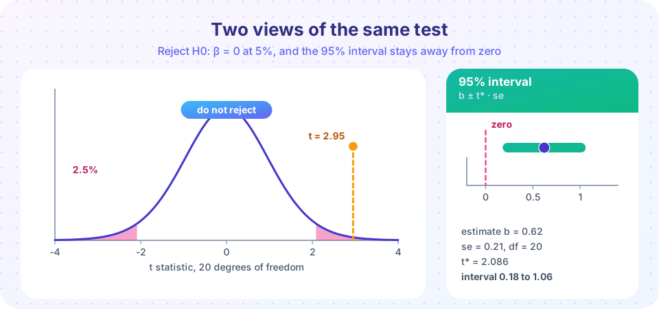
An estimated schooling coefficient is b = 0.62 with se = 0.21 and 20 degrees of freedom. Then t = 0.62 / 0.21 ≈ 2.95. Since 2.95 > 2.086 (the 5% critical value), we reject H0: β = 0 at the 5% level. We can also test other nulls. For H0: β = 1, t = (0.62 − 1) / 0.21 ≈ −1.81; |−1.81| < 2.086, so we do not reject that the true return is 1.
One-sided tests
If theory says an effect can only be positive, use H1: β > 0. You reject only when t is large and positive, using a critical value that puts the whole 5% in one tail (1.72 for 20 degrees of freedom, smaller than the two-sided 2.09). One-sided tests are more powerful in the stated direction, but you must choose the direction before seeing the data. Switching to a one-sided test after seeing a positive estimate is a form of cheating.
p-values
Comparing with a critical value gives a yes or no. The p-value gives more. It is the probability, assuming H0 is true, of obtaining a t statistic at least as extreme as the one observed. A p-value of 0.008 means: if the true coefficient were zero, only about 0.8% of samples would produce a statistic that extreme. Small p-values are evidence against H0. The decision rule is: reject if p < α.
Report p-values as numbers, not just stars. Two cautions shape their use.
- A p-value is not the probability that H0 is true. It is a probability about the data given H0, not about H0 given the data.
- A p-value of 0.049 and 0.051 are practically the same evidence, although they sit on opposite sides of 5%. Treating 0.05 as a cliff encourages bad practice.
Confidence intervals
A 95% confidence interval for βj is
bj ± t* · se(bj)
where t* is the 5% two-sided critical value. For example 2 above: 0.62 ± 2.086 × 0.21 = 0.62 ± 0.44, or about (0.18, 1.06). For example 1: 0.8 ± 3.182 × 0.346 = 0.8 ± 1.10, i.e. (−0.30, 1.90).
The interval and the test are two views of the same information. A two-sided 5% test of H0: β = c rejects exactly when c lies outside the 95% interval. The interval in example 1 contains zero, consistent with failing to reject. The interval in example 2 excludes zero and includes 1, consistent with both of our tests.
Intervals are more informative than a bare significant-or-not verdict, because they show the plausible size. An interval from 0.01 to 1.23 and one from 0.60 to 0.64 both exclude zero, but they tell very different stories about precision and about how much the effect could matter.
What "95%" means
The 95% refers to the procedure: if you could repeat the sampling many times and build an interval each time, about 95% of the intervals would contain the true value. For any one computed interval, the truth is either in it or not. Saying "there is a 95% probability that β is in (0.18, 1.06)" is a common shortcut but not the correct statement in this framework.
Statistical versus economic significance
A coefficient is statistically significant if its t statistic is large relative to the critical value. It is economically significant if its size matters for the question. They are different things.
- With millions of observations, a coefficient of 0.0003 dollars can be highly significant and economically irrelevant.
- With 30 observations, a coefficient of 5 dollars per hour can fail to be significant and still be of huge importance; the sample just cannot pin it down.
Always report the size, its interval and your judgment of whether it matters. A fixation on stars is a mark of the novice.
Multiple testing and "p-hacking"
If you test 20 unrelated variables at the 5% level, you expect about one to appear "significant" by pure chance. The probability that at least one is significant is 1 − 0.95²⁰ ≈ 64%. Researchers who run many specifications and report only those with stars produce unreliable results, a practice called p-hacking. Decide the main specification in advance, report all that you tried, and adjust for multiple comparisons when you test many hypotheses.
Common misconceptions
"A significant coefficient is a large coefficient." Significance depends on the ratio of estimate to standard error, which depends on sample size.
"Not significant means no effect." It may mean the sample is too small to detect the effect. Look at the confidence interval.
"The p-value is the probability that the null is true." It is the probability of data this extreme if the null were true.
"A 95% interval has a 95% chance of containing the truth, once computed." The 95% describes the long-run behavior of the procedure.
Try it
First example: compute the t statistic, p-value and 95% interval for both worked examples with scipy, and confirm the critical values quoted above.
Press Run (or Ctrl + Enter) to see the result here.
Program input · what you'd type while the program runs
Type the answers before you press Run, one per line. Each time the program reads a line (with input()), it gets the next line from this box.
Second example: see what "95%" means. We draw 100 samples from a population with a known mean, build a 95% interval from each, and count how many contain the truth. Intervals that miss are drawn in pink.
Press Run (or Ctrl + Enter) to see the result here.
Program input · what you'd type while the program runs
Type the answers before you press Run, one per line. Each time the program reads a line (with input()), it gets the next line from this box.
Third example: the multiple-testing trap. We regress an outcome on 20 completely irrelevant variables, test each at the 5% level, and repeat the experiment many times.
Press Run (or Ctrl + Enter) to see the result here.
Program input · what you'd type while the program runs
Type the answers before you press Run, one per line. Each time the program reads a line (with input()), it gets the next line from this box.
Check your understanding
Quick check · 5 questions
of 5 answered You scored / 5 · perfect!
-
1. An estimate b = 1.5 with se = 0.5 gives t = 3 for H0: β = 0. With 40 degrees of freedom, at the 5% two-sided level you
The two-sided 5% critical value with 40 degrees of freedom is about 2.02, and 3 exceeds it. -
2. A 95% confidence interval for a coefficient is (−0.30, 1.90). Which statement is consistent?
The interval contains zero, so a two-sided 5% test does not reject zero. -
3. What is a p-value?
It is a probability about the data under the null, not about the null itself. -
4. With 20 independent tests at the 5% level on irrelevant variables, the chance of at least one false 'significant' result is about
1 − 0.95^20 ≈ 0.64. -
5. A very large sample yields a highly significant coefficient of 0.0003 dollars. This is
Significance depends on precision, not on practical size.
Summary
- The t statistic is
(bj − c)/se(bj); under the classical assumptions it has a t distribution withn − k − 1degrees of freedom. - Reject when
|t|exceeds the critical value, or equivalently when the p-value is below α. - A 95% interval
bj ± t*·secontains exactly the null values that a two-sided 5% test does not reject. - p-values are probabilities about the data under H0, not about H0.
- Report effect sizes with intervals, distinguish statistical from economic significance and beware multiple testing.
Track your progress
Create a free account to tick off lessons and pick up where you left off on any device.
of Econometrics lessons completed