


















Lesson 48 of 49 · Projects and Practice
Cheat sheet: tests, fixes and designs
A one-page recap of chapters 5 to 8: formulas, tests, repairs and identifying assumptions, plus a Python calculator for the most common quantities.
This page is a quick reference for the second half of the course. It is built for the moment when you are looking at a regression and ask: what should I check, and what do I do about it? Read the picture first, then use the tables for formulas and thresholds. Everything here is explained in detail in the lessons; this page only reminds you.
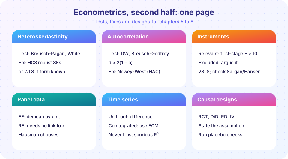
What you will learn
- The one-line version of each method from chapters 5 to 8.
- The formulas and thresholds you will use most.
- A calculator that evaluates them.
Key terms
Diagnose, then repair. Each problem has a signature symptom, a test and a repair. Identifying assumption. The untestable claim that turns an estimate into a causal one. Robust by default. Report robust or clustered standard errors unless you have a reason not to.
Errors: variance and memory
| Problem | Symptom | Test | Repair |
|---|---|---|---|
| Heteroskedasticity | Funnel in residuals vs fitted | Breusch-Pagan: LM = n R²_aux, df = number of auxiliary slopes. White: add squares and cross-products |
HC3 robust SEs; WLS with weights 1/σi²; log the outcome |
| Autocorrelation | Long runs of same-sign residuals | Durbin-Watson d ≈ 2(1 − ρ̂); Breusch-Godfrey (valid with lagged y) |
Newey-West HAC; add dynamics; Cochrane-Orcutt |
| Both | Time-series data with uneven variance | The two tests above | HAC errors |
Key facts: slopes remain unbiased (with exogenous regressors); the usual SEs, t and F tests are not. Sandwich: (X'X)⁻¹ [Σ ei² xi xi'] (X'X)⁻¹. Bartlett weights in HAC: wl = 1 − l/(L + 1), with L ≈ floor(4 (T/100)^(2/9)).
Endogeneity and instruments
| Item | Formula or rule |
|---|---|
| Omitted variable bias | plim b1 = β1 + β2 δ1 |
| Attenuation | plim b1 = β1 × Var(x*) / (Var(x*) + Var(v)) |
| Simple IV | Cov(z, y) / Cov(z, x) = reduced form / first stage |
| 2SLS | (X' P_Z X)⁻¹ X' P_Z y; use SEs from residuals with the actual x |
| Relevance | First-stage F well above 10 (robust version if heteroskedastic) |
| Validity (overidentified) | Sargan or Hansen J, df = excluded instruments − endogenous regressors |
| Endogeneity test | Hausman, or add the first-stage residual and test its coefficient |
| Weak-IV bias | Toward OLS; consider LIML or Anderson-Rubin intervals |
| Exclusion violation | Bias ≈ γ / π for a direct effect γ and first-stage slope π |
Panels and time series
| Topic | Rule |
|---|---|
| Error components | yit = xit'β + αi + uit; pooled OLS inconsistent if αi is correlated with x |
| Fixed effects | Within transformation; drops time-invariant regressors; cluster by unit |
| Random effects | Quasi-demeaning with θ = 1 − √(σu² / (σu² + T σα²)); needs αi unrelated to x |
| Hausman | H = (b_FE − b_RE)² / (Var_FE − Var_RE), chi-square under H0; reject means FE |
| Stationarity | Constant mean and variance; autocovariance depends on the lag only |
| Unit root | φ = 1; ADF critical values: constant −2.86, constant and trend −3.41 (5%) |
| Spurious regression | R² > DW is a warning for levels regressions |
| Cointegration | Engle-Granger: regress in levels, test the residual (about −3.34 at 5% for two variables); ECM with α < 0 |
| AR(1) forecast | μ + φʰ (yT − μ); variance σ² (1 − φ²ʰ)/(1 − φ²) |
Causal designs
| Design | Assumption | Checks |
|---|---|---|
| RCT | Random assignment, SUTVA, low attrition | Balance table; ITT; power |
| DiD | Parallel trends | Event study, placebo dates, cluster by unit |
| RD | Continuity at the cutoff | Density, covariate jumps, placebo cutoffs, bandwidths |
| IV / fuzzy RD | Relevance, exclusion, monotonicity | First stage, argument |
| Selection on observables | No unobserved confounders | Sensitivity analysis |
Naive difference = ATT + selection bias. ITT divided by the take-up gives the LATE under one-sided noncompliance.
Calculator
The functions below evaluate the formulas on this page. Edit the numbers at the bottom for your own problem.
Press Run (or Ctrl + Enter) to see the result here.
Program input · what you'd type while the program runs
Type the answers before you press Run, one per line. Each time the program reads a line (with input()), it gets the next line from this box.
How to use the sheet on a real problem
Work from the outside in. First decide whether the question is causal or descriptive, because that determines how worried you should be about endogeneity. Then look at the data structure: a cross-section points to heteroskedasticity and clustering by group, a panel to unit effects and within-unit dependence, a long time series to stationarity and autocorrelation. Only then choose the estimator, and finish by choosing the standard errors that match the structure. When two rows of a table seem to apply, as with a panel of macro variables that is both clustered and persistent, combine the repairs rather than picking one: for example, fixed effects with standard errors clustered by unit, or a cointegration check before differencing. Keep a short log of each specification you try and which diagnostic motivated it. That log becomes the robustness section of your write-up and protects you from the temptation to report only the version that looks best.
A last checklist before you submit a regression
- Did I plot the residuals?
- Which standard errors am I reporting, and are they appropriate for this data (robust, clustered, HAC)?
- Could a regressor be correlated with the error? If so, what is my argument or my instrument?
- If it is panel data, did I think about unit effects and clustering?
- If it is time series, did I check stationarity?
- What is the identifying assumption for any causal claim, and what evidence did I show?
- Whose effect am I estimating?
Common misconceptions
"A cheat sheet replaces understanding." It reminds you of formulas; deciding which one applies still needs the reasoning from the lessons.
"Rules of thumb are laws." F above 10, the 5% level and the Durbin-Watson zones are conventions. Look at the evidence, not just the threshold.
Check your understanding
Quick check · 4 questions
of 4 answered You scored / 4 · perfect!
-
1. A Durbin-Watson statistic of 2.0 corresponds to a first-order autocorrelation of about...
d is roughly 2(1 - rho); d = 2 means rho is about zero. -
2. Which pair is correctly matched?
RD relies on continuity of potential outcomes at the threshold. -
3. The sandwich estimator replaces the unknown error variances with...
Squared OLS residuals estimate the middle matrix consistently. -
4. With a first-stage F of 4, you should...
F below 10 flags weakness.
Summary
- Variance problems (heteroskedasticity, autocorrelation) get robust or modelled errors; endogeneity gets instruments or designs.
- Panels use FE or RE chosen by the Hausman logic and clustered errors; time series need stationarity checks and cointegration when relevant.
- Causal designs stand on identifying assumptions; show the checks.
- Use the calculator for quick numbers, and always say whose effect you estimate.
Next: Further study
Track your progress
Create a free account to tick off lessons and pick up where you left off on any device.
of Econometrics lessons completed