


















Lesson 13 of 49 · Simple and Multiple Regression
Goodness of fit and R-squared
Learn how the variation in y splits into explained and unexplained parts, how to compute and interpret R-squared and the standard error of regression, and why a high R-squared can mislead.
Once you have fitted a line, a natural question follows: how well does it describe the data? Two people can run the same regression and disagree: one says "the fit is excellent", the other "it explains little". To settle such arguments econometricians use a few standard measures. The most famous is R-squared, the share of the variation in the outcome that the model accounts for.
R-squared is easy to compute and easy to misuse. This lesson shows exactly what it measures, how it relates to the correlation you already know, which companion number tells you the typical size of the prediction miss, and why a high R-squared neither proves a theory nor guarantees a useful model.
What you will learn
- The three sums of squares: TSS, ESS and RSS, and how they relate.
- How to compute and interpret
R², and its link to correlation. - What the standard error of the regression measures.
- Why a high or low R-squared is not the final word on a model.
Key terms
Total sum of squares (TSS): Σ (yi − ȳ)², the total variation in y around its mean.
Explained sum of squares (ESS): Σ (ŷi − ȳ)², the variation captured by the fitted line.
Residual sum of squares (RSS or SSR): Σ ûi², the variation left over.
R-squared: R² = ESS / TSS = 1 − RSS / TSS.
Standard error of the regression (SER): the typical size of a residual, √(RSS / (n − 2)) in simple regression.
Splitting the variation
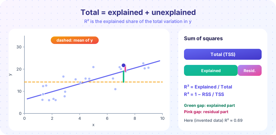
How much do the values of y vary? Measure variation around the mean of y. For observation i, the deviation yi − ȳ can be split into two parts:
yi − ȳ  =  (ŷi − ȳ)  +  (yi − ŷi)
 total     explained     residual
The explained part is how far the fitted line lifts the prediction from the overall mean; the residual part is what the line misses. In the picture, they are the green and pink gaps. Squaring and summing over all observations gives the central identity of regression:
TSS = ESS + RSS
The cross terms vanish because OLS residuals are uncorrelated with the fitted values (a property from Lesson 1). This identity holds for OLS with an intercept; it is why the decomposition is tidy.
R-squared
The coefficient of determination is the explained share of the total variation:
R² = ESS / TSS = 1 − RSS / TSS
It lies between 0 and 1. R² = 0 means the fitted line does no better than predicting ȳ for everyone (the slope is zero). R² = 1 means all points lie exactly on the line.
Worked example
Return to the five points from the previous lesson: x = 1..5, y = 1, 3, 2, 5, 4, with fitted line ŷ = 0.6 + 0.8x and residuals −0.4, 0.8, −1.0, 1.2, −0.6.
ȳ = 3, soTSS = (1−3)² + (3−3)² + (2−3)² + (5−3)² + (4−3)² = 4 + 0 + 1 + 4 + 1 = 10.RSS = 3.6(computed last lesson).ESS = TSS − RSS = 6.4. You can verify: fitted values1.4, 2.2, 3.0, 3.8, 4.6minus 3 give−1.6, −0.8, 0, 0.8, 1.6, whose squares sum to2.56 + 0.64 + 0 + 0.64 + 2.56 = 6.4.R² = 6.4 / 10 = 0.64.
The line accounts for 64% of the variation in y in this sample.
R-squared and correlation
In simple regression, R² is the squared sample correlation between x and y: R² = r². Here r = Σ(x−x̄)(y−ȳ) / √(Σ(x−x̄)² · Σ(y−ȳ)²) = 8 / √(10 · 10) = 0.8, and 0.8² = 0.64, matching. In multiple regression, R² equals the squared correlation between y and the fitted values ŷ.
The standard error of the regression
R-squared is a relative measure with no units. Often you want an absolute one: how far off, in the units of y, is a typical prediction? The standard error of the regression (SER, also called the residual standard error or root mean squared error) answers:
σ̂ = √( RSS / (n − k − 1) )
where k is the number of regressors (here k = 1). The denominator n − k − 1 accounts for the fitted coefficients: dividing by n would understate the typical error because the line was chosen to fit these very points, the same reasoning that gave us n − 1 for the sample variance. In the example σ̂ = √(3.6 / 3) = √1.2 ≈ 1.10: predictions miss by about 1.1 units in a typical case.
SER and R-squared answer different questions. Suppose wages are in dollars. A regression with R² = 0.05 and σ̂ = 4 tells you that schooling explains little of the variation and that a prediction is typically off by about 4 dollars. A model with a high R-squared can still have a large SER if y varies enormously to begin with.
What R-squared can and cannot do
It can describe how closely the sample hugs the line, compare models for the same dependent variable on the same data, and indicate how useful a model is for prediction.
It cannot tell you:
- Whether the model is correct. A badly misspecified model can have a high R-squared, and a correct one a low R-squared if the outcome is inherently noisy. Individual wages are shaped by countless factors, so cross-sectional wage regressions typically have modest R-squared values; time series of trending quantities often have values near 1.
- Whether a coefficient is causal. The fit says nothing about causation. You can have a high R-squared and a thoroughly biased slope.
- Whether the effect is important. A slope can matter a lot even if R-squared is low; one variable among many noisy influences still has the effect it has.
- Whether you can compare across different outcomes. R-squared from a regression of wage cannot be compared with R-squared from a regression of log wage, because the total variation being explained differs.
R-squared never falls when you add a variable
Add any regressor, even a column of random noise, and the in-sample R² will not decrease; usually it creeps up. So a higher R-squared can result from overfitting. The adjusted R-squared, which penalizes extra regressors, is covered in the next lesson on multiple regression.
Spurious regression with trends
Two unrelated series that both trend upward over time (say, the number of mobile phones and the price of cheese) can give an R-squared close to 1 when regressed on each other. The fit comes from the shared trend, not from any relationship. This "spurious regression" problem, identified by Clive Granger and Paul Newbold in the 1970s, is a central warning in time series econometrics (Chapter 7).
Common misconceptions
"A high R² proves my theory." It shows only that the model fits. Many theories, including wrong ones, produce high fits.
"A low R² means the regression is useless." Predicting human behavior is hard. A regression can estimate a precise, important average effect while explaining little of the individual-level variation.
"R² can be compared across any regressions." Only regressions with the same dependent variable and, ideally, the same sample are comparable.
Try it
First example: compute the three sums of squares, R² and SER for the worked example, and confirm that R² equals the squared correlation.
Press Run (or Ctrl + Enter) to see the result here.
Program input · what you'd type while the program runs
Type the answers before you press Run, one per line. Each time the program reads a line (with input()), it gets the next line from this box.
Second example: R-squared depends on how much noise surrounds the line, even when the slope is exactly the same. We keep the true slope at 2 and raise the noise.
Press Run (or Ctrl + Enter) to see the result here.
Program input · what you'd type while the program runs
Type the answers before you press Run, one per line. Each time the program reads a line (with input()), it gets the next line from this box.
Third example: the spurious regression trap. We generate 1,000 pairs of completely independent random walks (running sums of noise, which wander like trends) and report their R-squared when regressed on each other. Typical values are far above what independence would suggest.
Press Run (or Ctrl + Enter) to see the result here.
Program input · what you'd type while the program runs
Type the answers before you press Run, one per line. Each time the program reads a line (with input()), it gets the next line from this box.
Check your understanding
Quick check · 5 questions
of 5 answered You scored / 5 · perfect!
-
1. If TSS = 200 and RSS = 50, what is R²?
R² = 1 − RSS/TSS = 1 − 50/200 = 0.75. -
2. In a simple regression, R² equals
With one regressor, R² is the square of the sample correlation between x and y. -
3. What does the standard error of the regression measure?
It is √(RSS/(n − k − 1)), a typical prediction miss in the units of the outcome. -
4. Adding an irrelevant random variable to a regression will typically
In-sample R² never falls when a regressor is added, so it is not a reliable guide to model quality. -
5. Which conclusion is justified by R² = 0.05 in a wage regression on schooling?
A low R² reflects that many other factors affect wages; it does not rule out an important average effect.
Summary
TSS = ESS + RSSfor OLS with an intercept, andR² = ESS/TSS = 1 − RSS/TSS.- In simple regression
R²equals the squared correlation ofxandy. - The standard error of the regression
√(RSS/(n−k−1))gives the typical residual in the units ofy. - A high R-squared does not prove a model correct, a slope causal or an effect important; trending series can produce spurious fits.
- In-sample R-squared never falls when regressors are added; adjusted R-squared corrects for that.
Next: Multiple regression
Track your progress
Create a free account to tick off lessons and pick up where you left off on any device.
of Econometrics lessons completed