


















Lesson 18 of 49 · Inference and Specification
Gauss-Markov and the classical assumptions
Learn the classical linear model assumptions MLR.1 to MLR.6, why OLS is unbiased and BLUE, how to derive the variance and standard error of a slope, and what each assumption buys you.
OLS can be computed from any data, whether or not it deserves your trust. The formulas always return a line. Whether that line is a sensible estimate of anything depends on assumptions about how the data were generated. The classical linear model collects the assumptions under which OLS has attractive properties: it is unbiased, it has the smallest variance among a broad class of competitors, and, with one more assumption, its t and F statistics follow exact known distributions.
This lesson states the assumptions, shows why each is needed, derives the variance of the slope in simple regression and explains the Gauss-Markov theorem. It is the logical backbone of the chapter: every later problem, from heteroskedasticity in Chapter 5 to endogeneity in Chapter 6, is the story of one of these assumptions failing.
What you will learn
- The assumptions MLR.1 to MLR.6 and their meaning.
- Why OLS is unbiased under MLR.1 to MLR.4.
- The variance and standard error of the OLS slope, and what makes it small.
- What the Gauss-Markov theorem says: BLUE under MLR.1 to MLR.5.
Key terms
Unbiased: the average of the estimates over repeated samples equals the true parameter.
Efficient (best): has the smallest variance among the estimators being compared.
Homoskedasticity: the error variance is the same for all values of the regressors.
Exogeneity: the regressors are unrelated to the error term; formally E[u | x] = 0.
BLUE: Best Linear Unbiased Estimator.
The assumptions
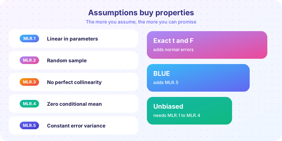
Write the population model y = β0 + β1·x1 + ... + βk·xk + u. Following a standard labeling:
MLR.1, linear in parameters. The model is linear in the βs, as you saw last chapter; transformed regressors are allowed.
MLR.2, random sampling. The observations (xi1, ..., xik, yi) are drawn independently from the population. This fits cross-sectional surveys; for time series and panels it must be modified (Chapter 7).
MLR.3, no perfect collinearity. No regressor is an exact linear combination of the others, and each varies in the sample. Otherwise X′X cannot be inverted. Note that high (but not perfect) correlation among regressors is allowed.
MLR.4, zero conditional mean (exogeneity). E[u | x1, ..., xk] = 0. Knowing the regressors tells you nothing about the average of the unobserved factors. This is the assumption that carries all the weight in applied work. If an omitted factor such as ability moves with schooling, MLR.4 fails.
MLR.5, homoskedasticity. Var(u | x1, ..., xk) = σ²: the spread of the errors does not depend on the regressors. If wages are more dispersed for highly educated workers than for others, this fails.
MLR.6, normality. The error u is independent of the regressors and normally distributed. It is needed only for exact small-sample t and F distributions; in large samples the central limit theorem makes it unnecessary.
Unbiasedness (MLR.1 to MLR.4)
Take simple regression and substitute the model for y into the slope formula. Because Σ(xi − x̄) = 0, the formula simplifies to
b1 = β1 + Σ (xi − x̄)·ui / Σ (xi − x̄)²
The estimate equals the truth plus an error term made of the unobserved us, weighted by the deviations of x. Taking expectations conditional on the observed xs, and using E[ui | x] = 0 from MLR.4, the second term vanishes:
E[b1 | x] = β1
So b1 is unbiased. The same argument works in multiple regression. Notice exactly where each assumption entered: MLR.1 to write the model, MLR.2 to treat observations separately, MLR.3 so the formula exists (variation in x), and MLR.4 to eliminate the error term on average. If MLR.4 fails because u is correlated with x, the second term does not average out and the estimate is biased, no matter how large the sample.
The variance of the slope (adding MLR.5)
How far from β1 is b1 likely to be? From the expression above, the variability of b1 is driven by the errors. Under MLR.5 the conditional variance is
Var(b1 | x) = σ² / Σ (xi − x̄)²
Three lessons follow.
- More noise (σ² larger) means less precision. If other factors scatter wages widely, you learn less.
- More variation in
xmeans more precision.Σ(xi − x̄)²is the total variation in the regressor. A regression of wages on schooling is more precise when your sample includes people with very different amounts of schooling than when everyone has 12 years. - More observations means more precision. The sum grows with
n, so the variance falls roughly like1/n.
In multiple regression the variance of bj becomes σ² / [SSTj · (1 − Rj²)], where SSTj is the total variation in xj and Rj² is the R-squared from regressing xj on the other regressors. The factor 1 − Rj² is the share of xj that is independent of the other regressors, which links back to partialling out: the less independent variation, the larger the variance. We return to this in the multicollinearity section of the last lesson of this chapter.
Estimating σ² and the standard error
The error variance σ² is unknown, but the residuals reveal it. The unbiased estimator is
σ̂² = RSS / (n − k − 1)
(the squared standard error of the regression from last chapter). Substituting gives the standard error of the slope:
se(b1) = σ̂ / √Σ(xi − x̄)²
Worked example
For the five-point example (x = 1..5, y = 1, 3, 2, 5, 4), earlier we found RSS = 3.6, n = 5, k = 1, Σ(x − x̄)² = 10.
σ̂² = 3.6 / 3 = 1.2, soσ̂ ≈ 1.095.Var(b1) ≈ 1.2 / 10 = 0.12, sose(b1) = √0.12 ≈ 0.346.
The slope estimate 0.8 therefore comes with a standard error of about 0.35, a ratio of about 2.3. Next lesson turns that ratio into a test.
The Gauss-Markov theorem
Under MLR.1 to MLR.5, OLS is BLUE: it has the smallest variance among all estimators that are linear in y and unbiased. That is the Gauss-Markov theorem. No cleverly weighted alternative within that class beats OLS.
The theorem has limits worth remembering. It compares only linear unbiased estimators; a biased estimator with lower variance (such as ridge regression) can have lower mean squared error, and nonlinear estimators can beat OLS if errors are far from normal (heavy tails, for instance). It also requires homoskedasticity; if MLR.5 fails, OLS remains unbiased but is no longer best, and the usual standard errors are wrong (Chapter 5).
Normality and exact inference (adding MLR.6)
If the errors are normal, b1 is exactly normal, and (b1 − β1)/se(b1) follows a t distribution with n − k − 1 degrees of freedom. That is the foundation of the t test in the next lesson. If errors are not normal, the CLT delivers approximately the same result when n is large, which is why the same tests are used in practice even though real wage errors are not exactly normal.
What each assumption protects
| Assumption fails | OLS unbiased? | Standard errors valid? | Chapter |
|---|---|---|---|
| MLR.3 (perfect collinearity) | cannot be computed | no estimate | 3 and 4 |
| MLR.4 (omitted factor, reverse causation) | no | invalid | 4 and 6 |
| MLR.5 (heteroskedasticity) | yes | no | 5 |
| MLR.2 (dependence, e.g. autocorrelation) | yes | no | 5 and 7 |
| MLR.6 (non-normal errors) | yes | approximately, for large n | this chapter |
Most threats to credible work come from MLR.4, because nothing in your data can check it: the error u is unobserved, and OLS residuals are by construction uncorrelated with the regressors. Defending MLR.4 requires economic reasoning and research design.
Common misconceptions
"Unbiased means close to the truth." Unbiased means right on average over repeated samples. Any single estimate can be far off, as the standard error indicates.
"Residuals that look uncorrelated with x show that MLR.4 holds." They are uncorrelated by construction, always. MLR.4 concerns the unobserved error, which you cannot see.
"OLS is the best estimator, period." It is best among linear unbiased estimators under MLR.1 to MLR.5. Outside those conditions, other estimators may be better.
"Large samples fix bias." More data shrink the variance, not the bias from a failing MLR.4.
Try it
First example: a Monte Carlo experiment. We simulate 5,000 samples from a model that satisfies MLR.1 to MLR.5 and check unbiasedness and the variance formula σ² / Σ(x − x̄)². The regressor values are held fixed across samples (as in the conditional-on-x statement of the theorem).
Press Run (or Ctrl + Enter) to see the result here.
Program input · what you'd type while the program runs
Type the answers before you press Run, one per line. Each time the program reads a line (with input()), it gets the next line from this box.
Second example: break MLR.4. The true model has an omitted variable z that is correlated with x. The short regression (leaving z out) is biased, and the bias does not shrink as the sample grows.
Press Run (or Ctrl + Enter) to see the result here.
Program input · what you'd type while the program runs
Type the answers before you press Run, one per line. Each time the program reads a line (with input()), it gets the next line from this box.
Third example: precision depends on the sample size and on how spread out x is. We compute the standard error of the slope for several designs.
Press Run (or Ctrl + Enter) to see the result here.
Program input · what you'd type while the program runs
Type the answers before you press Run, one per line. Each time the program reads a line (with input()), it gets the next line from this box.
Check your understanding
Quick check · 5 questions
of 5 answered You scored / 5 · perfect!
-
1. Which assumption is essential for OLS to be unbiased?
Exogeneity removes the error's contribution to b1 on average; homoskedasticity and normality affect variance and inference. -
2. Under MLR.1 to MLR.5, the Gauss-Markov theorem says OLS is
BLUE: smallest variance among linear unbiased estimators. -
3. Which change makes the OLS slope less precise?
Var(b1) = σ²/Σ(x − x̄)²; a larger σ² raises it. -
4. In the worked example, with RSS = 3.6, n = 5, k = 1 and Σ(x − x̄)² = 10, the standard error of the slope is about
σ̂² = 3.6/3 = 1.2, Var(b1) = 1.2/10 = 0.12 and se = √0.12 ≈ 0.346. -
5. If MLR.5 (homoskedasticity) fails but MLR.1 to MLR.4 hold, OLS is
Heteroskedasticity affects variance and the standard errors, not unbiasedness.
Summary
- MLR.1 to MLR.4 make OLS unbiased; MLR.5 gives a simple variance formula and the Gauss-Markov theorem; MLR.6 gives exact t and F tests.
b1 = β1 + Σ(x − x̄)u / Σ(x − x̄)²: bias arises exactly whenuis related tox.Var(b1) = σ²/Σ(x − x̄)²; the standard error isσ̂/√Σ(x − x̄)², withσ̂² = RSS/(n − k − 1).- OLS is BLUE under MLR.1 to MLR.5; outside them, other estimators or corrections may be better.
- The assumption you most need to defend, and cannot test directly, is MLR.4.
Track your progress
Create a free account to tick off lessons and pick up where you left off on any device.
of Econometrics lessons completed