


















Lesson 47 of 49 · Projects and Practice
Glossary: heteroskedasticity to causal designs
A plain-language glossary of the terms from the second half of the course: robust errors, instruments, panels, unit roots, cointegration and causal designs.
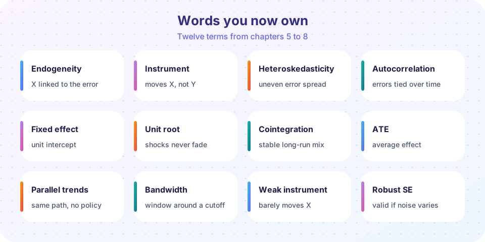
Econometrics is full of names that sound alike and mean different things. "Exogenous", "exclusion" and "exogeneity" are neighbours; "stationary", "trend-stationary" and "difference-stationary" look similar but call for different treatments. This glossary collects the terms from chapters 5 to 8, defined in a sentence or two each, with a pointer to where the idea appears.
What you will learn
- Quick, precise definitions for the key terms of chapters 5 to 8.
- Which terms are easy to confuse, and how to tell them apart.
- A searchable list you can use while studying.
Key terms
Convention. Terms are listed in alphabetical order. A symbol such as ρ or θ is explained where it is used. When two terms are easy to mix up, the entry says so.
A to C
ADF test (augmented Dickey-Fuller). A test whose null hypothesis is a unit root; it adds lagged differences to absorb serial correlation. Critical values are non-standard (chapter 7).
Anticipation. Units change behaviour before a policy starts, which contaminates pre-treatment periods in difference-in-differences.
ATE, ATT. The average treatment effect over the population, and over those actually treated.
Attenuation bias. Shrinkage of a slope toward zero caused by classical measurement error in a regressor.
Autocorrelation (serial correlation). Correlation between errors in different periods; it makes the usual standard errors unreliable (chapter 5).
Bandwidth. The distance from the cutoff within which observations are used in a regression discontinuity analysis; also the lag truncation in HAC estimation.
Breusch-Godfrey test. An LM test for autocorrelation of any order that remains valid with lagged dependent variables.
Breusch-Pagan test. An LM test for heteroskedasticity based on regressing squared residuals on regressors.
Cluster-robust standard errors. Standard errors that allow arbitrary correlation of errors within groups, such as units in a panel or states in a policy study.
Cointegration. A stationary linear combination of I(1) series, describing a stable long-run relationship (chapter 7).
Compliers. Units whose treatment status is changed by the instrument; IV and fuzzy RD estimate effects for them.
Continuity assumption. The condition for regression discontinuity: expected potential outcomes do not jump at the cutoff.
Counterfactual. The outcome that would have occurred under the alternative treatment status; it is never observed for the same unit.
D to H
Difference-in-differences (DiD). The change in the treated group minus the change in the control group, identified under parallel trends.
Durbin-Watson statistic. d ≈ 2(1 − ρ̂), a first-order test of autocorrelation; invalid when a lagged dependent variable is a regressor.
Endogeneity. A regressor is correlated with the error term, so OLS is biased and inconsistent (chapter 6).
Error correction model (ECM). A model of changes that includes last period's deviation from the long-run relationship, with an adjustment coefficient that should be negative.
Event study. Estimates of an effect for each period relative to the start of treatment; used to check pre-trends and to trace dynamics.
Exclusion restriction. The instrument affects the outcome only through the endogenous regressor. It cannot be tested with a single instrument.
Exogenous variable. A variable uncorrelated with the error term. Do not confuse this with a variable being "outside the model".
First stage. The regression of the endogenous regressor on the instruments and exogenous controls.
First-stage F. The F statistic for the excluded instruments; a value well above 10 is the minimum for a strong instrument.
Fixed effects (within estimator). OLS on data demeaned by unit; it removes time-invariant unobserved heterogeneity (chapter 7).
Fuzzy regression discontinuity. A design in which crossing the cutoff changes the probability of treatment rather than assigning it; estimated as an IV ratio.
GLS and FGLS. Generalized and feasible generalized least squares: OLS on transformed data that has constant variance and uncorrelated errors, with the transformation estimated in the feasible version.
HAC (Newey-West). Heteroskedasticity and autocorrelation consistent standard errors for time-series data.
Hausman test. A comparison of two estimators (FE versus RE, or OLS versus IV); a significant difference signals that the efficient one is inconsistent.
Heteroskedasticity. The variance of the error depends on the regressors (chapter 5). The opposite is homoskedasticity.
HC standard errors. White's heteroskedasticity-consistent covariance estimators, HC0 to HC3; HC3 is the recommended small-sample version.
I to R
Instrument. A variable that is relevant (moves the endogenous regressor) and excluded (affects the outcome only through it).
Integrated of order d, I(d). A series that is stationary after d differences; a random walk is I(1).
Intention-to-treat (ITT). The effect of being assigned to treatment, regardless of compliance.
J test (Sargan or Hansen). A test of overidentifying restrictions: do all instruments agree?
LATE. The local average treatment effect: the average effect for compliers.
Local linear regression. Fitting straight lines on each side of a cutoff within a bandwidth; the standard RD estimator.
LM test. A test based on n × R² from an auxiliary regression, compared with a chi-square distribution.
Measurement error (classical). Observed x = x* + v, noise uncorrelated with the truth.
Omitted variable bias. The bias β2 δ1 from leaving out a variable that affects the outcome and is correlated with an included regressor.
Overidentification. Having more instruments than endogenous regressors, which makes a validity test possible.
Panel data. Observations on the same units over several periods.
Parallel trends. The assumption that without treatment the groups would have changed by the same amount.
Placebo test. Running the method where the true effect is known to be zero, to look for evidence that the design is broken.
Potential outcomes. Y(1) and Y(0): the outcome with and without treatment.
Random effects. A panel estimator that treats the unit effect as uncorrelated with the regressors; efficient but inconsistent if that fails.
Random walk. yt = yt−1 + εt; shocks are permanent and the variance grows with time.
Reduced form. The regression of the outcome directly on the instruments and controls.
Running variable. The score that determines treatment in a regression discontinuity.
S to W
Sandwich estimator. A covariance estimator of the form bread × meat × bread, the basis of robust standard errors.
Selection bias. The difference between treated and untreated units in their outcomes without treatment.
Simultaneity. Two variables determined jointly, each affecting the other; a source of endogeneity.
Spurious regression. A regression between independent nonstationary series that shows a significant relationship.
Stationarity (weak). Constant mean, constant variance and autocovariances that depend only on the lag.
SUTVA. No spillovers between units and a single version of the treatment.
Trend-stationary. Stationary around a deterministic trend; detrend rather than difference.
Two-stage least squares (2SLS). Regress the endogenous variable on the instruments, then the outcome on the fitted values (with the correct standard errors).
Unit root. An autoregressive root equal to one; shocks never die out.
Weak instrument. An instrument with little first-stage power, causing bias toward OLS and unreliable inference.
Weighted least squares (WLS). OLS with weights equal to inverse error variances; efficient under known heteroskedasticity.
Within variation. Change in a variable over time for the same unit; fixed effects uses only this.
Pairs people confuse
- Heteroskedasticity versus endogeneity. The first is about the variance of the error; the second about its correlation with a regressor. One damages standard errors, the other the coefficients.
- Autocorrelation versus unit root. Autocorrelation can be present in a stationary process; a unit root is the extreme case with an autoregressive coefficient of one.
- Fixed versus random effects. Both model the unit effect; random effects assumes it is uncorrelated with the regressors.
- ITT versus LATE. ITT is the effect of the offer for everyone; LATE rescales it to those who comply.
- Sharp versus fuzzy RD. In a sharp design treatment switches on completely at the cutoff; in a fuzzy design only the probability jumps.
Try it: search the glossary
The widget below lets you filter a selection of the terms by typing. It is a small demonstration written in plain HTML and JavaScript, not a replacement for the full list above.
Check your understanding
Quick check · 4 questions
of 4 answered You scored / 4 · perfect!
-
1. Which term describes the effect of being assigned to treatment, regardless of compliance?
Intention-to-treat compares groups by assignment. -
2. Which statement distinguishes trend-stationary from difference-stationary series?
A deterministic trend is removed by regression on time; a stochastic trend (unit root) by differencing. -
3. The exclusion restriction says that the instrument...
The instrument's only route to the outcome runs through the regressor. -
4. Which statement about HC3 is correct?
HC3 divides squared residuals by (1 - h) squared and is recommended in small samples.
Summary
- Many pairs of terms look alike but are about different things: variance versus bias, autocorrelation versus unit roots, ITT versus LATE.
- Keep the list of identifying assumptions handy: exogeneity and exclusion for IV, parallel trends for DiD, continuity for RD.
- Use the glossary alongside the cheat sheet while practising.
Next: Cheat sheet
Track your progress
Create a free account to tick off lessons and pick up where you left off on any device.
of Econometrics lessons completed