


















Lesson 26 of 49 · Violations: Heteroskedasticity and Autocorrelation
Robust errors and weighted least squares
Repair inference under heteroskedasticity: the sandwich formula, the HC0 to HC3 family, weighted least squares and feasible GLS, with Python code.
You have found a funnel, a test has rejected constant variance, and you cannot ignore it. What now? There are two families of remedies, and they answer different questions.
The first asks: "I do not know the shape of the variance. Can I still get honest standard errors from OLS?" The answer, due to Eicker, Huber and White, is yes: heteroskedasticity-robust standard errors change nothing about the slopes and fix the standard errors. The second asks: "I do know (or can estimate) how the variance behaves. Can I use that to get a more precise estimate?" The answer is weighted least squares (WLS) and its feasible cousin, FGLS. This lesson builds both and tells you when to pick which.
What you will learn
- The sandwich formula for the OLS covariance matrix, and why it is robust.
- The differences between HC0, HC1, HC2 and HC3.
- How weighted least squares works, and why it can beat OLS.
- How feasible GLS estimates the weights, and what happens if the variance model is wrong.
Key terms
Sandwich estimator: a covariance estimator of the form bread × meat × bread. Leverage hi: the diagonal element of the hat matrix, measuring how far an observation's regressors are from the average. WLS: OLS on data where each observation is multiplied by a weight 1/σi. FGLS: feasible generalized least squares, which uses estimated variances. Clustering: allowing errors to be correlated within groups; a related extension of the sandwich idea.
The sandwich formula
Write the model in matrix form y = Xβ + u. The OLS estimator is b = (X'X)⁻¹X'y, and its exact sampling covariance is
Var(b | X) = (X'X)⁻¹ X' Ω X (X'X)⁻¹
where Ω is the covariance matrix of the errors. Under classical assumptions Ω = σ²I, the middle collapses, and the familiar σ²(X'X)⁻¹ remains. Under heteroskedasticity without correlation, Ω is diagonal with entries σi². The two outer terms are the "bread"; the middle X'ΩX is the "meat".
The key insight of White (1980): you do not need to estimate each σi² accurately (impossible with one observation each). You only need a good estimate of the single matrix X'ΩX = Σ σi² xi xi'. Replace σi² by the squared residual ei². Each ei² is a poor estimate of its own σi², but their weighted sum converges to the right matrix as n grows. That gives the HC0 estimator:
V_HC0 = (X'X)⁻¹ [ Σ ei² xi xi' ] (X'X)⁻¹
For a simple regression slope this reduces to Σ (xi − x̄)² ei² / [Σ (xi − x̄)²]², the empirical counterpart of the true variance formula from the previous lesson.
The HC family
Squared residuals are too small on average, especially for high-leverage points (the OLS line is pulled toward them, so their residuals shrink). Small-sample fixes rescale the residuals:
| Name | Squared-residual term | Comment |
|---|---|---|
| HC0 | ei² |
White's original; fine in large samples |
| HC1 | ei² × n/(n − k) |
Degrees-of-freedom correction; Stata's robust |
| HC2 | ei² / (1 − hi) |
Unbiased under constant variance |
| HC3 | ei² / (1 − hi)² |
Conservative; recommended for small samples |
Long and Ervin (2000) and MacKinnon and White (1985) found HC3 to perform best when n is below a few hundred. In big samples, all four agree closely. The robust standard errors are consistent without any model for the variance. The price is that they are valid only in large samples, and the robust t statistic needs more observations than the usual one to follow its reference distribution.
Press Run (or Ctrl + Enter) to see the result here.
Program input · what you'd type while the program runs
Type the answers before you press Run, one per line. Each time the program reads a line (with input()), it gets the next line from this box.
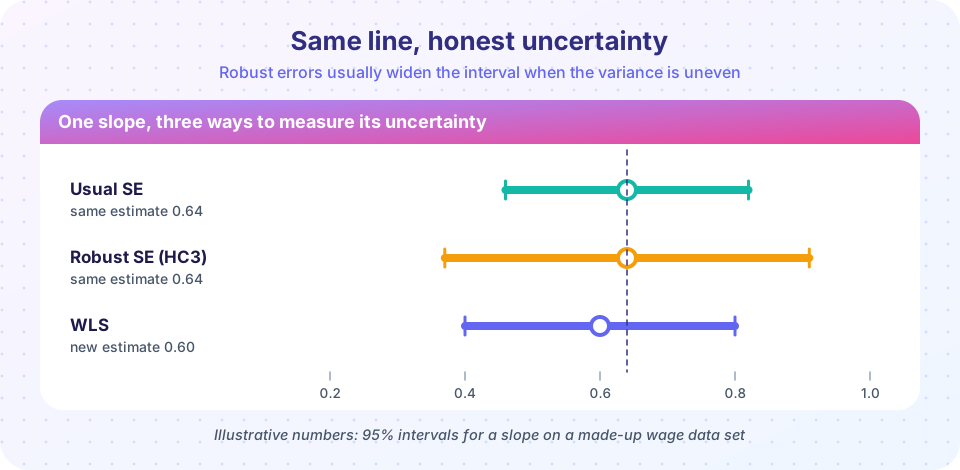
All five numbers describe the same slope. The usual standard error assumes a constant spread; the other four let the spread vary and generally agree with one another.
Weighted least squares
Suppose the error variance of observation i is known up to a constant: Var(ui | xi) = σ² hi, with hi a known positive number. For example, if yi is a city average of ni households, then hi = 1/ni. Dividing the whole equation by √hi gives
yi/√hi = β0 (1/√hi) + β1 (xi/√hi) + ui/√hi
and the transformed error ui/√hi has variance σ², which is constant. Applying OLS to the transformed data is weighted least squares, with weights wi = 1/hi. It minimizes Σ wi (yi − b0 − b1xi)²: observations with small variance count for more. In matrix form b_WLS = (X'WX)⁻¹ X'Wy with W = diag(wi).
If the weights are correct, Gauss-Markov applies to the transformed model, so WLS is BLUE and its usual standard errors are valid. The gain over OLS can be large when the variance changes a lot.
When do you actually know the form? Rarely, except in averaged data (hi = 1/ni), in data where each observation is a sum of mi independent contributions (hi = mi) or in some designs where variance is proportional to a known size variable.
Feasible GLS
If the form is unknown but plausible, estimate it. A standard recipe for Var(u|x) = σ² exp(δ0 + δ1x1 + ... ):
- Fit OLS and save residuals
e. - Regress
log(e²)on the regressors and obtain the fitted valuesĝ. - Set
ĥ = exp(ĝ)and weightsŵ = 1/ĥ. - Run WLS with weights
ŵ.
Feasible GLS is not unbiased in small samples, because the weights depend on the data, but it is consistent and asymptotically efficient if the variance model is right. The warning: if the variance model is wrong, FGLS is still consistent but no longer efficient, and its usual standard errors may be wrong. Many careful applied economists therefore report WLS or FGLS estimates together with robust standard errors, which protects against a misspecified weighting scheme.
Press Run (or Ctrl + Enter) to see the result here.
Program input · what you'd type while the program runs
Type the answers before you press Run, one per line. Each time the program reads a line (with input()), it gets the next line from this box.
Both histograms should centre on 0.5. The WLS histogram is narrower, which is the efficiency gain the Gauss-Markov theorem promised for the transformed model.
Which one should I use?
- Default for cross-section applied work: OLS with HC3 (or HC1 in large samples). It needs no assumption about the variance.
- Known weights: WLS. Use it for averages and aggregates, and report robust errors too.
- Strong dependence on a size variable, suspect functional form: first try a log transformation of
y; it often removes the funnel entirely and gives coefficients with a percentage interpretation. - Time series: use HAC errors, covered in the serial correlation lesson.
Common misconceptions
"Robust standard errors change my coefficients." They do not. Only the standard errors, t statistics, p-values and intervals change.
"Robust errors are always larger." Usually, but not always; in some samples they are smaller. They are valid, not simply bigger.
"WLS with guessed weights is always safe." Wrong weights keep consistency but can lose efficiency and distort the usual standard errors. Pair it with robust errors.
Check your understanding
Quick check · 5 questions
of 5 answered You scored / 5 · perfect!
-
1. Which estimator changes only the standard errors, leaving OLS coefficients untouched?
HC standard errors reuse the OLS slopes and fix only the covariance estimate. -
2. In the sandwich formula, what replaces the unknown error variances?
Each squared residual is a noisy stand-in for sigma squared of that observation; their weighted sum estimates the middle matrix well. -
3. Which HC version is usually recommended when the sample is small?
HC3 corrects squared residuals for leverage and tends to perform best in small samples. -
4. City averages are computed from n_i households each. Which weights does WLS use if the household-level error variance is constant?
The variance of an average is sigma squared over n_i, so the weight is the inverse, n_i. -
5. FGLS is consistent if...
Misspecified weights keep consistency under the mean assumption but lose efficiency, so robust errors remain advisable.
Summary
- The sandwich estimator
(X'X)⁻¹ [Σ ei² xi xi'] (X'X)⁻¹gives valid standard errors without modelling the variance; HC3 is the safe small-sample choice. - WLS divides each observation by its error standard deviation, giving efficient estimates when the weights are right.
- FGLS estimates the weights from residuals; it is consistent but only as good as its variance model.
- A good default is OLS with robust errors; use WLS when the weights come from the data's structure.
Next: Serial correlation
Track your progress
Create a free account to tick off lessons and pick up where you left off on any device.
of Econometrics lessons completed