


















Lesson 42 of 49 · Causal Methods and Practice
Regression discontinuity
Learn sharp and fuzzy regression discontinuity: the continuity assumption, local linear estimation, bandwidth choice and the validity checks that matter.
Rules create thresholds. A student with an entrance exam score of 70 gets a scholarship; one with 69 does not. A town with a population of at least 5,000 must hire a second police officer; one with 4,999 need not. A firm with 50 workers faces extra regulation; one with 49 does not. Rules like these treat nearly identical units differently, and that is a gift to the empirical researcher.
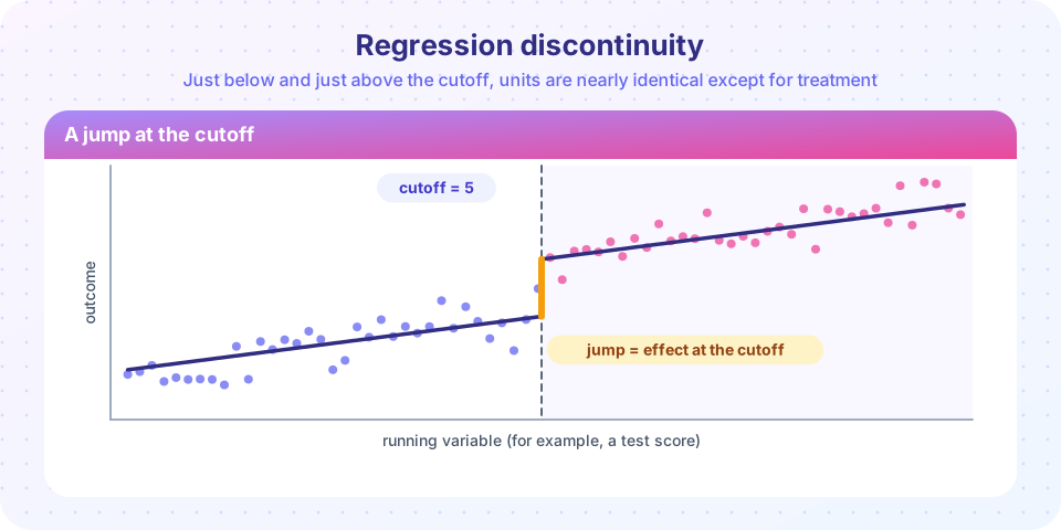
A regression discontinuity (RD) design exploits this. Units just below and just above the cutoff are almost the same in everything except the treatment, so a jump in the outcome right at the cutoff can be attributed to the treatment. Thistlethwaite and Campbell introduced the idea in 1960, and it became one of the most credible non-experimental designs after Imbens, Lemieux and others formalized it in the 2000s.
What you will learn
- The sharp RD estimand and the continuity assumption that identifies it.
- How local linear regression estimates the jump, and why bandwidth matters.
- The difference between sharp and fuzzy designs.
- The validity checks: density, covariate balance, placebo cutoffs and bandwidth sensitivity.
Key terms
Running variable X: the score that determines treatment (also called the forcing variable). Cutoff c: the threshold. Sharp RD: everyone above the cutoff is treated and nobody below. Fuzzy RD: crossing the cutoff only changes the probability of treatment. Bandwidth h: how far from the cutoff observations are used. Local estimate: the effect applies at the cutoff, not necessarily elsewhere.
The sharp design
Treatment is Di = 1 if Xi ≥ c and 0 otherwise. The effect at the cutoff is
τ = lim x↓c E[Y | X = x] − lim x↑c E[Y | X = x]
the jump in the conditional expectation of the outcome at c. The identifying assumption is continuity: the expected potential outcomes E[Y(0) | X = x] and E[Y(1) | X = x] are continuous functions of x at c. In words: absent treatment, nothing else would jump at the cutoff. The main threat is manipulation: if people can precisely control their score and the benefit is attractive, those just above the cutoff may differ from those just below. A student who can retake the test until she passes 70 is not the same as one who cannot.
Notice how local the claim is. RD identifies the effect for units at the cutoff. It may not apply to a student scoring 95.
Estimation: local linear regression
The standard method fits straight lines on each side of the cutoff using only observations within a window [c − h, c + h]:
Yi = α + τ Di + β1 (Xi − c) + β2 Di (Xi − c) + εi, for |Xi − c| ≤ h
The coefficient τ on the treatment dummy is the estimated jump. Letting the slope differ on each side (the interaction) is important: forcing equal slopes imposes a restriction that can create a false jump. Observations closer to the cutoff are often given more weight using a triangular kernel w = 1 − |X − c|/h.
Bandwidth choice is a bias-variance trade-off. A narrow window has little bias (the units are more alike and a line is a good approximation) but few observations and large variance. A wide window has more precision but more bias if the true relationship curves. Data-driven rules such as the Imbens-Kalyanaraman (2012) and Calonico-Cattaneo-Titiunik (2014) optimal bandwidths are the norm, with bias-corrected, robust confidence intervals; software implementing them is widely available. Always report how results change with the bandwidth.
Do not fit high-order global polynomials over the entire range of X. Gelman and Imbens (2019) showed they give noisy and misleading estimates because points far from the cutoff influence the fit at the cutoff. Local linear (or at most quadratic) fits are preferred.
Fuzzy designs
Sometimes crossing the cutoff only makes treatment more likely: a scholarship is offered above 70, but some eligible students decline and a few below it receive other support. In a fuzzy RD the cutoff acts as an instrument: the effect is the jump in the outcome divided by the jump in the probability of treatment,
τ_fuzzy = [jump in E(Y | X)] / [jump in E(D | X)]
This is the Wald estimator from chapter 6 evaluated at the cutoff, and it estimates a local effect for the compliers at the cutoff.
Checking validity
- Plot the data. Bin the running variable into small intervals, plot mean outcomes for each bin and look for a jump at the cutoff. If you cannot see it in the plot, be sceptical of a significant estimate.
- Density test. Check that the number of observations does not jump at the cutoff (McCrary, 2008; Cattaneo, Jansson and Ma, 2020). Bunching just above the cutoff suggests manipulation.
- Covariate balance. Pre-determined characteristics (age, previous grades) should not jump at the cutoff; run the same RD estimator with each as the outcome.
- Placebo cutoffs. Apply the estimator at fake cutoffs where nothing should happen (for example, at points away from the real one on the untreated side); no jumps should appear.
- Bandwidth and specification sensitivity. Vary the bandwidth, the kernel and the polynomial order; the estimate should be stable.
- Donut hole. Drop observations very close to the cutoff, where manipulation is most likely, and check whether results hold.
Local linear estimation in code
We simulate a scholarship that raises an outcome by 1.8 at a cutoff of 5, with a smooth curved relationship in the running variable. The function fits the weighted local linear regression and returns the jump, a robust standard error and the number of observations used.
Press Run (or Ctrl + Enter) to see the result here.
Program input · what you'd type while the program runs
Type the answers before you press Run, one per line. Each time the program reads a line (with input()), it gets the next line from this box.
All estimates should be close to 1.8, with standard errors shrinking as the window widens. With very wide windows the linear fit ignores the curvature in the simulated data, which introduces a little bias, which is the trade-off in action.
Sensitivity and falsification
The second program makes the standard diagnostics: a histogram of the running variable around the cutoff, the estimate as a function of the bandwidth, and placebo cutoffs at points where no treatment occurs.
Press Run (or Ctrl + Enter) to see the result here.
Program input · what you'd type while the program runs
Type the answers before you press Run, one per line. Each time the program reads a line (with input()), it gets the next line from this box.
The histogram is roughly flat across the cutoff, the estimate stays near 1.8 for all bandwidths (the error bars shrink as the window widens), and the placebo jumps are indistinguishable from zero. Those are the pictures you want to see in every RD paper.
Common misconceptions
"RD gives the average effect for everyone." It identifies the effect at the cutoff only. Extrapolating to units far away needs further assumptions.
"A higher-order polynomial fits better, so it is safer." High-order global polynomials give erratic estimates at the boundary; use local linear.
"If the score is a test, manipulation cannot happen." Retakes, rounding, appeals and strategic reporting can all create sorting around a threshold; always test the density.
"Fuzzy RD is just a worse sharp RD." It is a different estimand (a local effect for compliers) that rests on the same continuity argument plus IV conditions.
Check your understanding
Quick check · 5 questions
of 5 answered You scored / 5 · perfect!
-
1. The continuity assumption in RD states that...
Without treatment, nothing else would jump at the cutoff. -
2. A narrow bandwidth in local linear RD generally means...
Observations near the cutoff are more comparable (less bias) but there are fewer of them (more variance). -
3. In a fuzzy RD, the estimate equals...
The cutoff acts as an instrument; the effect is a Wald ratio at the cutoff. -
4. Bunching of observations just above the cutoff suggests...
A density jump indicates units may be sorting around the threshold. -
5. Which is a good placebo test for RD?
If the method finds 'effects' at fake cutoffs, the design is not credible.
Summary
- RD compares units just above and below a cutoff; the effect is the jump in the expected outcome at the threshold, identified by continuity of potential outcomes.
- Estimate with local linear regression on each side, choose bandwidth by a data-driven rule and show sensitivity; avoid high-order global polynomials.
- Fuzzy RD divides the outcome jump by the treatment-probability jump (IV at the cutoff).
- Validity checks: density test, covariate balance, placebo cutoffs, donut holes; the estimate is local to the cutoff.
Next: Chapter 8 review
Track your progress
Create a free account to tick off lessons and pick up where you left off on any device.
of Econometrics lessons completed