


















Lesson 38 of 49 · Panel Data and Time Series
Chapter 7 review: panel data and time series
Review chapter 7: a one-picture summary, a recap table, working Python tools for clustered fixed effects and unit-root decisions, and a ten-question quiz.
This chapter introduced two data structures and the one idea that unifies the dangers in both: what kind of variation drives your estimate? In a panel, you can choose between differences across units and changes within units, and the choice decides which unobserved traits contaminate the result. In a time series, you must check whether the variation comes from a stable stochastic process or from a persistent drift that makes ordinary inference collapse.
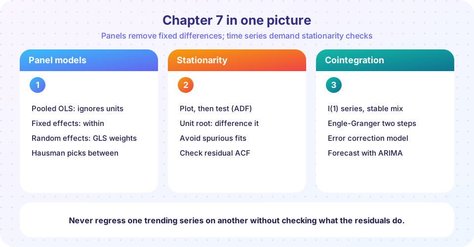
What you will learn
- A compact recap of fixed effects, random effects, stationarity and cointegration.
- Two practical tools: fixed effects with cluster-robust standard errors, and a unit-root decision helper.
- Ten mixed questions to test the chapter.
Key terms
Within estimator: OLS on unit-demeaned data. Hausman test: compares FE and RE estimates. Cluster-robust SE: valid under arbitrary within-unit correlation. I(1): needs one difference to become stationary. Cointegration: a stationary linear combination of I(1) series. ECM: error correction model.
Recap table
| Topic | Key formula or idea | Remember |
|---|---|---|
| Error components | yit = xit'β + αi + uit |
αi correlated with x makes pooled OLS inconsistent |
| Fixed effects | (yit − ȳi) = β (xit − x̄i) + ... |
Removes time-invariant traits; time-invariant regressors drop out |
| First differences | Δyit = β Δxit + Δuit |
Same as FE when T = 2 |
| Random effects | quasi-demeaning with θ |
Needs αi uncorrelated with x; Hausman or Mundlak checks it |
| Clustering | Sandwich with unit-level scores | Default for panels |
| Stationarity | constant mean, variance, autocovariances by lag | Needed for ordinary t tests |
| Unit root | φ = 1, shocks are permanent |
ADF null is a unit root; critical values are non-standard |
| Spurious regression | Independent I(1) series look related | R² > DW is a warning |
| Cointegration | yt − β xt is I(0) |
Engle-Granger; ECM with α < 0 |
| Forecasting | μ + φʰ (yT − μ), interval grows with h |
Judge out of sample |
Three connections between the two halves of the chapter:
- Dynamics matter in both. In a panel with
Tlarge, you must worry about serial correlation within units (cluster, or model the dynamics); in a long panel of macro variables you may also need unit-root tests. - Both are about what you hold constant. Fixed effects holds each unit constant; cointegration holds the long-run gap constant.
- Differencing is a blunt tool. First differences remove unit effects and unit roots, but they also remove information. Use them knowingly.
Tool 1: fixed effects with clustered standard errors
The function below computes the within estimator for one regressor and compares the classical standard error (which ignores serial correlation within units) with the cluster-robust one. The data are invented, with persistent errors within each unit.
Press Run (or Ctrl + Enter) to see the result here.
Program input · what you'd type while the program runs
Type the answers before you press Run, one per line. Each time the program reads a line (with input()), it gets the next line from this box.
With persistent errors inside each unit and a persistent regressor, the classical standard error is too small, and the cluster-robust one is noticeably larger. The slope itself is unchanged.
Tool 2: a unit-root decision helper
The helper runs an ADF test with a constant on the level and, if the unit root is not rejected, on the first difference, and prints the suggested treatment. It is a teaching sketch, not a complete decision procedure: always look at a plot too.
Press Run (or Ctrl + Enter) to see the result here.
Program input · what you'd type while the program runs
Type the answers before you press Run, one per line. Each time the program reads a line (with input()), it gets the next line from this box.
The stationary series passes. The other three are nonstationary by construction, but the last one is a transformed series, so look at what the output says and compare with a plot before deciding.
Common misconceptions
"Fixed effects solves all endogeneity." It removes only time-invariant confounders; time-varying ones remain.
"If a series is trending I should always difference it." Test for trend-stationarity and cointegration first.
"The Hausman test tells me which model is true." It tests one assumption about the unit effect.
Check your understanding
Quick check · 10 questions
of 10 answered You scored / 10 · perfect!
-
1. Fixed effects removes which kind of confounder?
The within transformation eliminates anything that is constant for a unit over time. -
2. Random effects is consistent only if...
RE treats alpha_i as part of the error and needs it to be unrelated to x. -
3. With T = 2, first differencing gives the same slope as...
With two periods, demeaning and differencing are equivalent. -
4. Cluster-robust standard errors in a panel allow for...
The sandwich is built from unit-level scores, so within-unit dependence is unrestricted. -
5. A random walk is...
One difference of a random walk is white noise, so the walk is integrated of order one. -
6. The ADF test has which null hypothesis?
ADF starts from a unit root and requires evidence to reject it. -
7. In an error correction model, alpha = -0.4 means...
A negative alpha pulls the system back toward equilibrium at that speed. -
8. Why use special critical values in the Engle-Granger test?
Estimating the cointegrating coefficient first makes the residuals look more stationary, so the critical values are more negative. -
9. A high R-squared and a very low Durbin-Watson statistic in a levels regression suggest...
This pattern is the signature of regressing independent nonstationary series. -
10. For a stationary AR(1), as the forecast horizon grows the point forecast...
The forecast of the deviation shrinks by the factor phi each period.
Summary
- Panels:
αicorrelated withxbreaks pooled OLS; fixed effects (within) fixes it; random effects needsαiunrelated tox; cluster standard errors by unit. - Time series: stationarity is the condition for ordinary inference; test unit roots with ADF, difference I(1) series, and use cointegration and ECMs when series share a long-run link.
- Forecast with stationary models and judge accuracy out of sample.
- Always ask which variation your estimate uses.
Track your progress
Create a free account to tick off lessons and pick up where you left off on any device.
of Econometrics lessons completed